Introduction: Scientific Background
Substantial Biophysical Damages Will Occur in the Absence of Strong Climate Policy Action
The world’s climate has already changed measurably in response to accumulating greenhouse gas (GHG) emissions. These changes as well as projected future disruptions have prompted intense research into the nature of the problem and potential policy solutions. This document aims to summarize much of what is known about both, adopting an economic lens focused on how ambitious climate objectives can be achieved at the lowest possible cost.
Considerable uncertainties surround both the extent of future climate change and the extent of the biophysical impacts of such change. Notwithstanding the uncertainties, climate scientists have reached a strong consensus that in the absence of measures to reduce GHG emissions significantly, the changes in climate will be substantial, with long-lasting effects on many of Earth’s physical and biological systems. The central or median estimates of these impacts are significant. Moreover, there are significant risks associated with low probability but potentially catastrophic outcomes. Although a focus on median outcomes alone warrants efforts to reduce emissions of GHGs, economists argue that the uncertainties and associated risks justify more aggressive policy action than otherwise would be warranted (Weitzman 2009; 2012).
The scientific consensus is expressed through summary documents offered every several years by the United Nations–sponsored Intergovernmental Panel on Climate Change (IPCC). These documents indicate the projected outcomes under alternative representative concentration pathways (RCPs) for GHGs (IPCC 2014). Each of these RCPs represents different GHG trajectories over the next century, with higher numbers corresponding to more emissions (see box 1 for more on RCPs).
Box 1. Representative Concentration Pathways (RCPs)
The expected path of GHG emissions is crucial to accurately forecasting the physical, biological, economic, and social effects of climate change. RCPs are scenarios, chosen by the IPCC, that represent scientific consensus on potential pathways for GHG emissions and concentrations, emissions of air pollutants, and land use through 2100. In their most-recent assessment, the IPCC selected four RCPs as the basis for its projections and analysis. We describe the RCPs and some of their assumptions below:
- RCP 2.6: emissions peak in 2020 and then decline through 2100.
- RCP 4.5: emissions peak between 2040 and 2050 and then decline through 2100.
- RCP 6.0: emissions continue to rise until 2080 and then decline through 2100.
- RCP 8.5: emissions rise continually through 2100.
The IPCC does not assign probabilities to these different emissions pathways. What is clear is that the pathways would require different changes in technology and policy. RCPs 2.6 and 4.5 would very likely require significant advances in technology and changes in policy in order to be realized. It seems highly unlikely that global emissions will follow the pathway outlined in RCP 2.6 in particular; annual emissions would have to start declining in 2020. By contrast, RCPs 6.0 and 8.5 represent scenarios in which future emissions follow past trends with minimal to no change in policy and/or technology.

The four RCPs imply different effects on global temperatures. Figure A indicates the projected increases in temperature associated with each RCP scenario (relative to preindustrial levels).1 The figure suggests that only the significant reductions in emissions underlying RCPs 2.6 and 4.5 can stabilize average global temperature increases at or around 2°C. Many scientists have suggested that it is critical to avoid increases in temperature beyond 2°C or even 1.5°C—larger temperature increases would produce extreme biophysical impacts and associated human welfare costs. It is worth noting that economic assessments of the costs and benefits from policies to reduce CO2 emissions do not necessarily recommend policies that would constrain temperature increases to 1.5°C or 2°C. Some economic analyses suggest that these temperature targets would be too stringent in the sense that they would involve economic sacrifices in excess of the value of the climate-related benefits (Nordhaus 2007, 2017). Other analyses tend to support these targets (Stern 2006). In scenarios with little or no policy action (RCPs 6.0 and 8.5), average global surface temperature could rise 2.9 to 4.3°C above preindustrial levels by the end of this century. One consequence of the temperature increase in these scenarios is that sea level would rise by between 0.5 and 0.8 meters (figure B).

Countries’ Relative Contributions to CO2 Emissions Are Changing
The extent of climate change is a function of the atmospheric stock of CO2 and other greenhouse gases, and the stock at any given point in time reflects cumulative emissions up to that point. Thus, the contribution a given country or region makes to global climate change can be measured in terms of its cumulative emissions.
Up to 1990, the historical responsibility for climate change was primarily attributable to the more-industrialized countries. Between 1850 and 1990, the United States and Europe alone produced nearly 75 percent of cumulative CO2 emissions (see figure C). Such historic responsibility has been a primary issue in debates about how much of the burden of reducing current and future emissions should fall on the shoulders of developed versus developing countries.
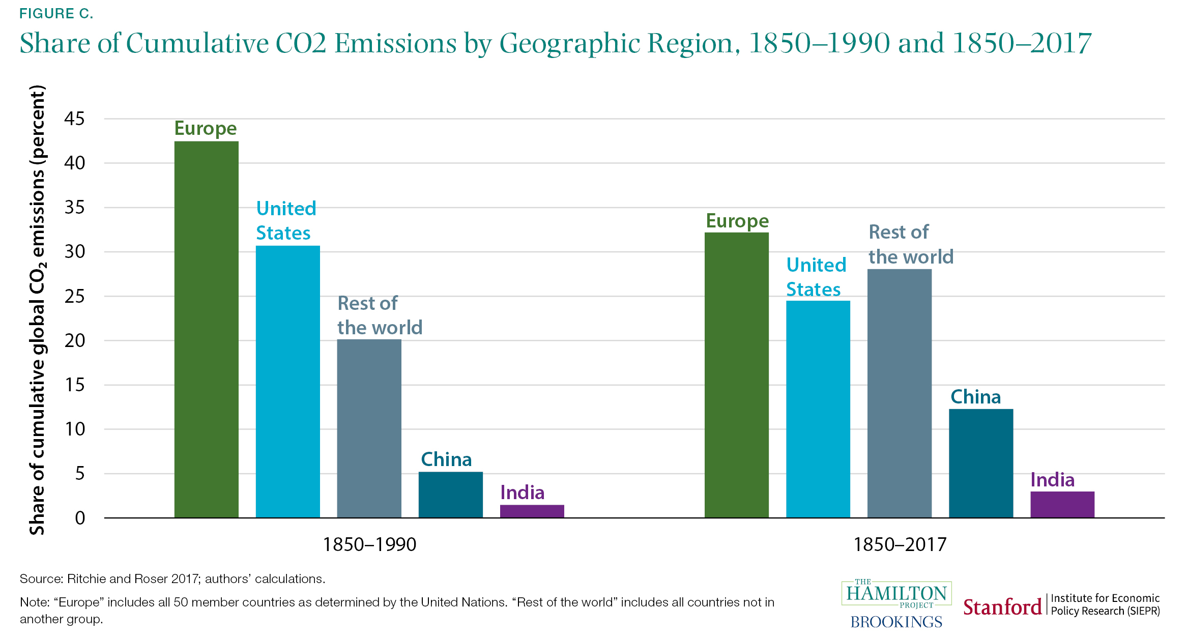
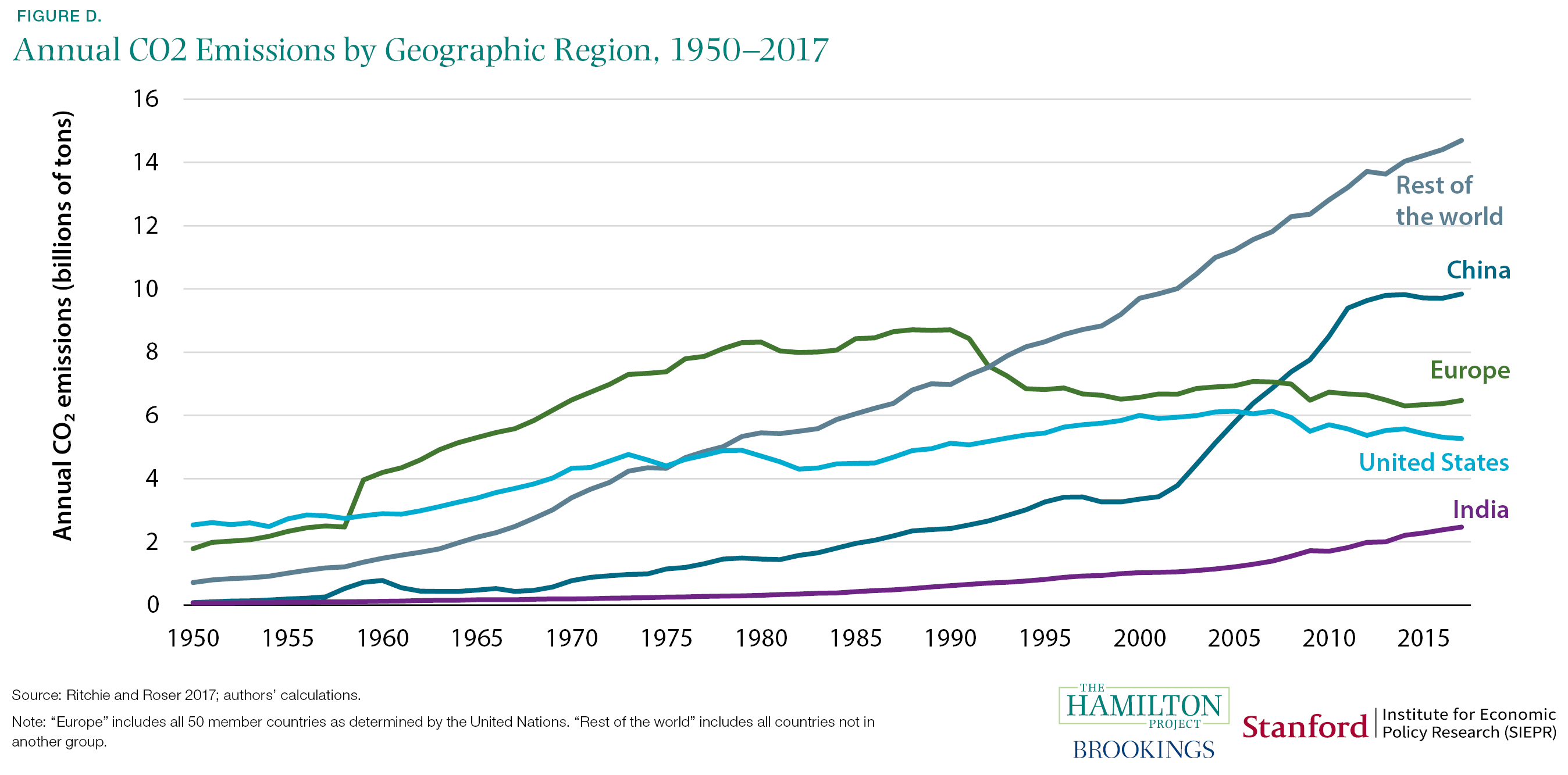
Although the United States and other developed nations continue to be responsible for a large share of the current excess concentration of CO2, relative contributions and responsibilities are changing. As of 2017, the United States and Europe accounted for just over 50 percent of cumulative CO2 emitted into the atmosphere since 1850. A reason for this sharp decline (as indicated in figures C and D) is that CO2 emissions from China, India, and other developing countries have grown faster than emissions from the developed countries (though amongst major economies, the United States has one of the highest rates of per capita emissions in the world and is far ahead of China and India [Joint Research Centre 2018]). Therefore, it seems likely that in order to avert the worst effects of climate change, emissions reduction efforts will be required by both historic contributors—the United States and Europe—as well as more recently developing countries such as China and India.
Nations’ Pledges under the Paris Agreement Imply Significant Reductions in Emissions, but Not Enough to Avoid a 2°C Warming
The future of climate change might seem dismal in light of the recent increase in global emissions as well as the potential future growth in emissions, temperatures, and sea levels under RCPs 6.0 and 8.5. Failure to take any climate policy action would lead to annual emissions growth rates far above those that would prevent temperature increases beyond the focal points of 1.5°C and 2°C (figure E). As indicated earlier, cost-benefit analyses in various economic models lead to differing conclusions as to whether it is optimal to constrain temperature increases to 1.5°C or 2°C (Nordhaus 2007, 2016; Stern 2006).2 Fortunately, countries have been taking steps to combat climate change, referred to in figure E as “Current policy” (which includes policy commitments made prior to the 2015 Paris Agreement). Comparing “No climate policies” and “Current policy” shows that the emissions reduction implied by current policies will lead to roughly 1°C lower global temperature by the end of the century. A large share of this lowered emission path is attributable to actions by states, provinces, and municipalities throughout the world.

Further reductions are implied by the 2015 Paris Agreement, under which 195 countries pledged to take additional steps. The Paris Agreement’s pledges, if met, would keep global temperatures 0.5°C lower than “Current policy” and about 1.5°C lower than “No climate policy” in 2100 (see figure E). Although this can be viewed as a positive outcome, a morenegative perspective is that these policies would still allow temperatures in 2100 to be 2.6 to 3.2°C above preindustrial levels—significantly above the 1.5 or 2.0°C targets that have become focal points in policy discussions.
In the following set of facts, we describe the costs of climate change to the United States and to the world as well as potential policy solutions and their respective costs.
Fact 1: Damages to the U.S. economy grow with temperature change at an increasing rate.
The physical changes described in the introduction will have substantial effects on the U.S. economy. Climate change will affect agricultural productivity, mortality, crime, energy use, storm activity, and coastal inundation (Hsiang et al. 2017).
In figure 1 we focus on the economic costs imposed by climate change in the United States for different cumulative increases in temperature. It is immediately apparent that economic costs will vary greatly depending on the extent to which global temperature increase (above preindustrial levels) is limited by technological and policy changes. At 2°C of warming by 2080–99, Hsiang et al. (2017) project that the United States would suffer annual losses equivalent to about 0.5 percent of GDP in the years 2080–99 (the solid line in figure 1). By contrast, if the global temperature increase were as large as 4°C, annual losses would be around 2.0 percent of GDP. Importantly, these effects become disproportionately larger as temperature rise increases: For the United States, rising mortality as well as changes in labor supply, energy demand, and agricultural production are all especially important factors in driving this nonlinearity.
Looking instead at per capita GDP impacts, Kahn et al. (2019) find that annual GDP per capita reductions (as opposed to economic costs more broadly) could be between 1.0 and 2.8 percent under IPCC’s RCP 2.6, and under RCP 8.5 the range of losses could be between 6.7 and 14.3 percent. For context, in 2019 a 5 percent U.S. GDP loss would be roughly $1 trillion.
There is, of course, substantial uncertainty in these calculations. A major source of uncertainty is the extent of climate change over the next several decades, which depends largely on future policy choices and economic developments—both of which affect the level of total carbon emissions. As noted earlier, this uncertainty justifies more aggressive action to limit emissions and thereby help insure against the worst potential outcomes.
It is also important to highlight what figure 1 leaves out. Economic effects that are not readily measurable are excluded, as are costs incurred by countries other than the United States. In addition, if climate change has an impact on the growth rate (as opposed to the level) of output in each year, then the impacts could compound to be much larger in the future (Dell, Jones, and Olken 2012).3

Fact 2: Struggling U.S. counties will be hit hardest by climate change.
The effects of climate change will not be shared evenly across the United States; places that are already struggling will tend to be hit the hardest. To explore the local impacts of climate change, we use a summary measure of county economic vitality that incorporates labor market, income, and other data (Nunn, Parsons, and Shambaugh 2018), paired with county level costs as a share of GDP projected by Hsiang et al. (2017).4
Figure 2 shows that the bottom fifth of counties ranked by economic vitality will experience the largest damages, with the bottom quintile of counties facing losses equal in value to nearly 7 percent of GDP in 2080–99 under the RCP 8.5 scenario (a projection that assumes little to no additional climate policy action and warming of roughly 4.3°C above preindustrial levels).5 Counties that will be hit hardest by climate change tend to be located in the South and Southwest regions of the United States (Muro, Victor, and Whiton 2019). Rao (2017) finds that nearly two million homes are at risk of being underwater by 2100, with over half of those being located in Florida, Louisiana, North Carolina, South Carolina, and Texas. More-prosperous counties in the United States are often in the Northeast, upper Midwest, and Pacific regions, where temperatures are lower and communities are less exposed to climate damage.
An important limitation of these estimates is that they assume that population in each county remains constant over time (Hsiang et al. 2017).6 To the extent that people will adjust to climate change by moving to less-vulnerable areas, this adjustment could help to diminish aggregate national damages but may exacerbate losses in places where employment falls. Moreover, the limited ability of low-income Americans to migrate in response to climate change exposes them to particular hardship (Kahn 2017).
The concentration of climate damages in the South and among low-income Americans implies a disproportionate impact on minority communities. Geographic disadvantage is overlaid with racial disadvantage (Hardy, Logan, and Parman 2018), and Black, Latino, and indigenous communities are likely to bear a disproportionate share of climate change burden (Gamble and Balbus 2016).

Fact 3: Globally, low-income countries will lose larger shares of their economic output.
Unlike other pollutants that have localized or regional effects, GHGs produce global effects. These emissions constitute a negative spillover at the widest scale possible: For example, emissions from the United States contribute to warming in China, and vice versa. Moreover, some places are much more exposed to economic damages from climate change than are other places; the same increase in atmospheric carbon concentration will cause larger per capita damages in India than in Iceland.
This means that carbon emissions and the damages from those emissions can be (and, in fact, are) distributed in very different ways. Figure 3 shows impacts on per capita GDP based on a study of the GDP growth effects of warming, highlighting the relatively high per capita income reductions in Latin America, Africa, and South Asia (though higher-income countries would lose more absolute aggregate wealth and output because of their higher levels of economic activity). The figure also uses a higher estimate of potential economic damages that takes into account impacts on productivity and growth that accumulate over time as opposed to looking at snapshots of lost activity in a given year. Thus, the estimates are higher than those presented in facts 1 and 2, highlighting both the uncertainty and the potentially disastrous outcomes that are possible.
Beyond showing the potentially destructive scale, this map suggests global inequity: Several of the regions that contribute relatively little to the climate change problem—regions with relatively low per capita emissions—nevertheless suffer relatively high climate damages per capita.

Fact 4: Increased mortality from climate change will be highest in Africa and the Middle East.
The reductions in economic output highlighted in fact 3 are not the only damages expected from climate change. One important example is the effect of climate change on mortality. In places that already experience high temperatures, climate change will exacerbate heat-related health issues and cause mortality rates to rise.
Figure 4 relies on estimates from Carleton et al. (2018) to show climate change’s expected effects on mortality in 2100. The geographical distribution of the impact on mortality is very uneven. Some of the most-significant impacts are in the equatorial zone because these locations are already very hot, and high temperatures become increasingly dangerous as temperatures rise further. For example, Accra, Ghana is projected to experience 160 additional deaths per 100,000 residents. In colder regions, mortality rates are sometimes predicted to fall, reflecting decreases in the number of dangerously cold days: Oslo, Norway is projected to experience 230 fewer deaths per 100,000. But for the world as a whole, negative effects are predominant, and on average 85 additional deaths per 100,000 will occur (Carleton et al. 2018).
Also evident in figure 4 is the role of income. Wealthier places are better able to protect themselves from the adverse consequences of climate change. This is a factor in projections of mortality risk from climate change: the bottom third of countries by income will experience almost all of the total increase in mortality rates (Carleton et al. 2018).
Mortality effects are disproportionately concentrated among the elderly population. This is true whether the effects are positive (when dangerously cold days are reduced) or negative (when dangerously hot days are increased) (Carleton et al. 2018; Deschenes and Moretti 2009).

Fact 5: Energy intensity and carbon intensity have been falling in the U.S. economy.
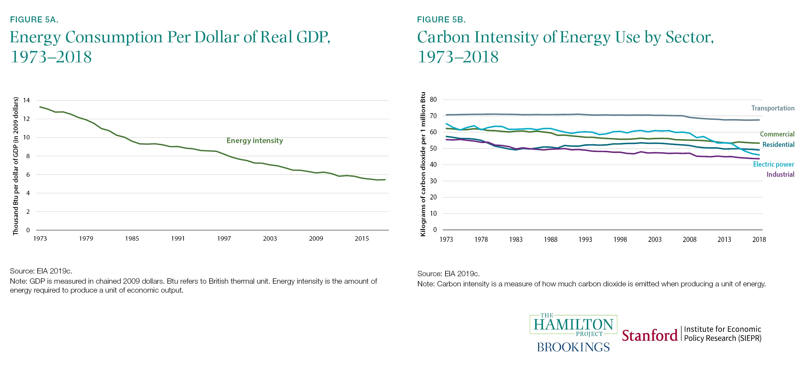
The high-damage climate outcomes described in previous facts are not inevitable: There are good reasons to believe that substantial emissions reductions are attainable. For example, not only has the emissions-to-GDP ratio of the U.S. economy declined over the past two decades, but during the last decade the absolute level of emissions has declined as well, despite the growth of the economy. From a peak in 2007 through 2017, U.S. carbon emissions have fallen 14 percent while output grew 16 percent (Bureau of Economic Analysis 2007–17; U.S. Environmental Protection Agency [EPA] 2007–17; authors’ calculations). This reversal was produced by a combination of declining energy intensity of the U.S. economy (figure 5a) and declining carbon intensity of U.S. energy use (figure 5b). However, emissions increased in 2018, which suggests that sound policy will be needed to continue making progress (Rhodium Group 2019).
U.S. energy intensity (defined as energy consumed per dollar of GDP) has been falling both in times of economic expansion and contraction, allowing the economy to grow even as energy use falls. This has been crucial for mitigating climate change damages (CEA 2017; Obama 2017). Some estimates suggest that declining energy intensity has been the biggest contributor to U.S. reductions in carbon emissions (EIA 2018). Technological advancements and energy efficiency improvements have in turn driven the reduction in energy intensity (Metcalf 2008; Sue Wing 2008).
At the same time that energy intensity has fallen, the carbon intensity of energy use has also fallen in each of the major sectors (shown in figure 5b). Improved methods for horizontal drilling have led to substantial increases in the supply of low-cost natural gas and less use of (relatively carbon-intensive) coal (CEA 2017).7 Technological advances have also helped substantially reduce the cost of providing power from renewable energy sources like wind and solar. From 2008 to 2015, roughly two thirds of falling carbon intensity in the power sector came from using cleaner fossil fuels and one third from an increased use of renewables (CEA 2017). Non-hydro-powered renewable energy has risen substantially over a short period of time, from 4 percent of all net electricity generation in 2009 to 10 percent in 2018 (EIA 2019a; authors’ calculations).
Fact 6: The price of renewable energy is falling.
The declining cost of producing renewable energy has played a key role in the trends described in fact 5. Figure 6 shows the declining prices of solar and wind energy—not including public subsidies—over the 2010–17 period. Because these price decreases have followed largely from technology induced supply increases, solar and wind energy now play a more-important role in the U.S. energy mix (CEA 2017). In many settings, however, clean energy remains more expensive on average than fossil fuels (The Hamilton Project [THP] and the Energy Policy Institute at the University of Chicago [EPIC] 2017), highlighting the need for continued technological advances.
The increasing share of renewables in energy supply is due in part to cost-reducing advances in technology and increased exploitation of economies of scale. Government subsidies—justified by the social costs of carbon emissions—for renewable energy have also played a role. When the negative spillovers from CO2 emissions are incorporated into the price of fossil fuels, many forms of clean energy are far cheaper than many fossil fuels (THP and EPIC 2017). However, making a much broader use of clean energy faces technological hurdles that have not yet been fully addressed. Renewable energy sources are in many cases intermittent—they make power only when the wind blows or the sun shines—and shifting towards more renewable energy production may require substantial improvements in battery technology and changes to how the electricity market prices variability (CEA 2016). The technological developments that drive falling clean energy prices are the product of public and private investments. In a Hamilton Project policy proposal, David Popp (2019) examines ways to encourage faster development and deployment of clean energy technologies.

Fact 7: Some emissions abatement approaches are much more costly than others.
There are many ways to reduce net carbon emissions, from better livestock management to renewable fuel subsidies to reforestation. Each of these abatement strategies comes with its own costs and benefits. To facilitate comparisons, researchers have calculated the cost per ton of CO2-equivalent emissions.8 We show high and low estimates of these average costs in figure 7, reproduced from Gillingham and Stock (2018).9
Less-expensive programs and policies include the Clean Power Plan—a since-discontinued 2014 initiative to reduce power sector emissions—as well as methane flaring regulations and reforestation. By contrast, weatherization assistance and the vehicle trade-in policy Cash for Clunkers are more expensive (see figure 7). It is important to recognize that some policies may have goals other than emissions abatement, as with Cash for Clunkers, which also aimed to provide fiscal stimulus after the Great Recession (Li, Linn, and Spiller 2013; Mian and Sufi 2012).
But when the goal is to reduce emissions at the lowest cost, economic theory and common sense suggest that the cheapest strategies for abating emissions should be implemented first. State and federal policy choices can play an important role in determining which of the options shown in figure 7 are implemented and in what order.
A common approach is to impose certain emissions standards—for example, a low-carbon fuel standard. The difficulty with this approach is that, in some cases, standards require abatement methods involving relatively high costs per ton while some low-cost methods are not implemented. This can reflect government regulators’ limited information about abatement costs or political pressures that favor some standards over others. By contrast, a carbon price—discussed in facts 8 through 10—helps to achieve a given emissions reduction target at the minimum cost by encouraging abatement actions that cost less than the carbon price and discouraging actions that cost more than that price.
However, policies other than a carbon price are often worthy of consideration. In a Hamilton Project proposal, Carolyn Fischer describes the situations in which clean performance standards can be implemented in a relatively efficient manner (2019).10

Fact 8: Numerous carbon pricing initiatives have been introduced worldwide, and the prices vary significantly.
At the local, national, and international levels, 57 carbon pricing programs have been implemented or are scheduled for implementation across the world (World Bank 2019). Figure 8 plots some of the key national and U.S. subnational initiatives,
showing carbon taxes in green and cap and trade in purple. By imposing a cost on emissions, a carbon price encourages activities that can reduce emissions at a cost less than the carbon price.
Immediately apparent from figure 8 is the wide range of the carbon prices, reflecting the range of carbon taxes and aggregate emissions caps that different governments have introduced. At the highest end is Sweden with its price of $126 per ton; by contrast, Poland and Ukraine have imposed prices just above zero.11 A sufficiently high carbon price would change the cost-benefit assessment of some existing nonprice policies, as described in a Hamilton Project proposal by Roberton Williams (2019).
A crucial question for policy is the appropriate level of a carbon price. According to economic theory, efficiency is maximized when the carbon price is equal to the social cost of carbon.12 In other words, a carbon price at that level would not only facilitate the adoption of the lowest-cost abatement activities (as discussed under fact 7) but would also achieve the level of overall emissions abatement that maximizes the difference between the climate-related benefits and the economic costs.13 Although setting the carbon price equal to the social cost of carbon maximizes net benefits, the monetized environmental benefits also exceed the economic costs when the carbon price is below (or somewhat above) the optimal value.
Estimates of the social cost of carbon depend on a wide range of factors, including the projected biophysical impacts associated with an incremental ton of CO2 emissions, the monetized value of these impacts, and the discount rate applied to convert future monetized damages into current dollars.14 As of 2016, the Interagency Working Group on Social Cost of Carbon—a partnership of U.S. government agencies—reported a focal estimate of the social cost of carbon (SCC) at $51 (adjusted for inflation to 2018 dollars) per ton of CO2 (indicated by the dashed line in figure 8).15

Fact 9: Most global GHG emissions are still not covered by a carbon pricing initiative.
Just as important as the carbon price is the share of global emissions facing the price. Many countries do not price carbon, and in many of the countries that do, important sources of emissions are not covered. When implementing carbon prices, policymakers have tended to start with the power sector and exclude some other emissions sources like energy-intensive manufacturing (Fischer 2019).
The carbon pricing systems that do exist are not evenly distributed across the world (World Bank 2019). Programs are heavily concentrated in Europe, Asia, and, to a lesser extent, North America. This distribution aligns roughly with the distribution of emissions, though the United States is an outlier: as discussed in the introduction, Europe has generated 33 percent of global CO2 emissions since 1850, the United States 25 percent, and China 13 percent (Ritchie and Roser 2017; authors’ calculations). According to currently scheduled and implemented initiatives, in 2020 the United States will be pricing only 1.0 percent of global GHG emissions; by comparison, Europe will be pricing 5.5 percent, and China will be pricing 7.0 percent (see figure 9).
Figure 9 shows each region’s priced emissions—including both implemented and planned (in 2020) carbon pricing—as a share of total global emissions. Between 2005 and 2012, the European Union’s cap and trade program was the only major carbon pricing program. However since the Paris Agreement, there has been a growing number of implemented and scheduled programs, with the largest of these being China’s national cap and trade program set to take effect in 2020. Despite this activity, it is likely that a carbon price will still not be applied to 80 percent of global emissions of GHGs in 2020 (World Bank 2019; authors’ calculations).

Fact 10: Proposed U.S. carbon taxes would yield significant reductions in CO2 and environmental benefits in excess of the costs.
To assess proposals for a national U.S. carbon price, it is important to understand the size of the likely emissions reduction. Figure 10 shows projections of emissions reductions from Barron et al. (2018) under different assumptions about the level and subsequent growth rate of a U.S. carbon price. Over the 2020-30 period a carbon tax starting at $25 per ton in 2020 and increasing at 1 percent annually above the rate of inflation achieves a reduction in CO2 of 10.5 gigatons, or an 18 percent reduction from the baseline (emissions level in 2005). A more-ambitious $50 per ton price, rising at 5 percent subsequently, would reduce near-term emissions by an estimated 30 percent.16
A major attraction of using carbon pricing to achieve emissions reductions (as compared to adopting standards and other conventional regulations for this purpose) is its ability to induce the market to adopt the lowest-cost methods for reducing emissions. As of late 2019, nine U.S. states participate in the Regional Greenhouse Gas Initiative (RGGI), in which electric power plants trade permits that currently have a market price of around $5.20 per short ton of carbon 10. Proposed U.S. carbon taxes would yield significant reductions in CO2 and environmental benefits in excess of the costs. (RGGI Inc. 2019).17 That means that electric power plants covered under the RGGI are able to find methods of emissions abatement at a cost of $5.20 per ton at the margin and would buy permits at that price rather than undertake any abatement opportunities at a higher cost. A lower aggregate cap—or a higher carbon tax—would continue to select for the abatement approaches that have the lowest costs per ton for a given sector.
Even at much higher levels, emissions pricing leads to environmental benefits—reduced climate and other environmental damages—that exceed the economic sacrifices involved (i.e., the expense of reducing emissions).18 A central estimate of the social cost of carbon (in 2018 dollars) is $51 per ton (Interagency Working Group on Social Cost of Carbon 2016). However, many recent proposals have tended to entail carbon prices below this level.19 Goulder and Hafstead (2017) find that a U.S. carbon tax of $20 per ton in 2019, increasing at 4 percent in real terms for 20 years after that, yields climate related benefits that exceed the economic costs by about 70 percent.20

The authors did not receive financial support from any firm or person for this article or from any firm or person with a financial or political interest in this article. None of the authors is currently an officer, director, or board member of any organization with a financial or political interest in this article.
Authors


-
Footnotes
- Each RCP embodies a different set of assumptions about emissions, as described in box 1. Each RCP was also formulated by a different modeling team drawing on different elements of the research literature. As such, the parameters of each RCP are not fully harmonized, and the range of RCP projections reflects both different modeling assumptions and different assumptions about emissions.
- It should be noted that the scenarios used to make emissions projections in figure E are not RCPs; hence they are different from the scenarios used in figures A and B. Instead, it uses policy scenarios outlined by the Climate Action Tracker.
The Brookings Institution is committed to quality, independence, and impact.
We are supported by a diverse array of funders. In line with our values and policies, each Brookings publication represents the sole views of its author(s).