
- Homepage
- Introduction
- Chapter 1: Which districts allocate resources progressively?
- Chapter 2: Does teacher sorting contribute to financial inequalities?
- Case studies: Massachusetts, Indiana, Louisiana, Nevada, New York, and North Carolina
- Methodological appendix
Data
Chapter 1
The main sources of school finance information are state-specific data files from the Edunomics NERD$ database. We focus on spending from the 2018-2019 school year. We use the normed total spending variable “pp_normed_nerds” for the nationwide analysis to make estimates more comparable across districts and states.
We complement these data with county-level income inequality information (Gini coefficient) from the American Community Survey (five-year estimates from 2015 to 2019). Additionally, we incorporate county-level election data from the MIT Election Lab. Specifically, we use Biden’s vote share in the 2020 presidential election in each county to measure political affiliation.
To transform county-level variables to the school-district level, we estimate the proportion of students from the district located in schools within each county. Most districts are located in just one county, in which case we assume all county measures apply to the district(s) contained in them. However, there are many exceptions where districts span multiple counties. In these cases, we construct the weighted average of the county-level information with the proportion of enrolled students of the district in each county. For example, if 75% of the students in a district are enrolled in a school in County A (where 60% voted for Biden) and 25% are enrolled in a school in County B (where 40% voted for Biden), then three-fourths of the weighted average of county statistics for that district would come from County A (i.e., for a weighted total of 55% voting for Biden).
We then bring in district-level community information from the NCES and ACS EDGE databases (5-year estimates from 2015 to 2019). This information includes community racial composition, percent of the population receiving SNAP benefits, and median income. We also merge district-level school segregation information from the Stanford Education Data Archive (SY 2017-2018).
We further complement this information with data from the NCES’s Common Core of Data (SY 2018-2019) detailing student enrollment and racial composition, the number of free-or-reduced priced lunch (FRPL)-eligible or directly certified students, district locale, and students with an Individualized Education Program (IEP).
Finally, we merge a sample of school board data from 300 randomly selected school districts across the four locale classifications in the Common Core of Data (city, suburban, town, and rural locations). More specifically, we restricted the sample to districts with at least 500 students enrolled and then randomly selected 25 districts from each of three sub-locale types for each locale (e.g., city-large, city-midsize, and city-small). We collected these data ourselves from school district and school board websites (e.g., to identify the number of seats on each board) as well as from county and state election results (e.g., to identify whether school board elections occurred on-cycle or off-cycle with other elections). We did this to ensure a broad representation of districts in a relatively small sample. Regression analyses involving school board data are weighted by district enrollment to prevent low-enrollment districts from getting disproportionate weight.
Chapter 2
Here, too, the primary sources of school finance information are the state-specific data files from the NERD$ database, reporting spending in the 2018-2019 school year. Some of the primary spending variables used in the analysis were included in the datasets, while others were created through simple computations. Appendix Table 1 presents the key spending variables that we use:
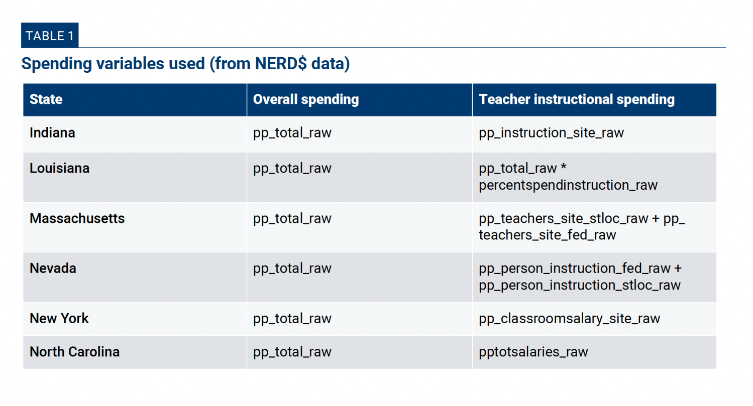
Chapter 2 conducts a within-state analysis, and because we are focusing on teacher salary and instructional spending, we do not use the normed variable. For robustness, we replicated our full analysis with the normed spending variable and did not find any notable differences in the analysis. The normed variable, however, yielded a more restricted sample for all sample states, particularly Nevada and New York, so we chose to focus on the raw total expenditures reported in the NERD$ data.
Next, we merge data from the Civil Rights Data Collection (CRDC) (2017-2018) with the NERD$ state files. The CRDC data provide school-level information on teacher staffing (e.g., the share of novice teachers and FTE counts for teachers and instructional support staff). We retain only observations that are common between the NERD$ and CRDC data, which exceeds 85% in all analysis states. This file is one academic year removed from other data sources, but it is the closest-in-time dataset available (CRDC collects data biannually).
Finally, we merge in data from the Common Core of Data (CCD) (2018-2019). The CCD data provide school-level information on student enrollment (e.g., FRPL), school type and level, and whether the school is in operation. We also incorporate NCES’s district-level comparable wage index to make dollars comparable across locations (within the same state). The wage index accounts for median wage differences in college-educated workers who are not working in education but are working within the same geographical region.
Trimming for the analysis samples
For both chapters we limit the sample to only regular public and vocational schools (excluding charter schools) serving primary, middle, and high school students. We drop schools identified in the NERD$ data as having problematic values or a student count of zero/missing.
We then trim our sample differently depending on the requirements of each chapter of the report. The differences in the sample between the two chapters are detailed below.
Chapter 1
To reduce the influence of extreme and potentially erroneous data points, we trim the top and bottom 1% of observations within each state for the state/local expenditure variable (which had not been normed or cleaned in the Edunomics data in the way the “pp_normed_nerds” variable had been).
To construct a progressivity ratio, we drop districts where either all or none of the students qualify for free-or-reduced price lunch or are directly certified. We do this because we cannot compare allocations for economically advantaged and disadvantaged students within districts that enroll students from one of these groups but not the other. We also drop schools in districts where the total number of schools is less than two (or where fewer than two schools have FRPL/direct certification information).
We use the percentage of FRPL-qualifying students as our measure of student poverty where available. We supplement this with the percentage of students directly certified where FRPL data are not available.
The final observation counts are: 8,667 for the sample with normed spending data (shown on the map), 8,132 for the sample with differentiated state/local and federal spending data (NH, OR, OH did not report on this dimension), and 8,435 districts with non-missing data from all incorporated sources. Our school board sample consists of 300 districts in total and 290 with non-missing data across all variables.
Chapter 2
We take several steps to ensure data quality in variables included in the analysis, particularly since we are not using the normed spending variable for this chapter. First, we drop all schools flagged in the NERD$ data as having suspect spending values at the school level. Second, we trim the top and bottom 1% of schools based on the teacher salary or instructional spending and overall spending values. Third, we flag schools in the top and bottom 1% of schools based on teacher FTEs and support staffing and teacher aide FTEs. We also flag the top 1% of schools on their percentage of novice teachers. We drop schools flagged as having extreme values on any of these variables.
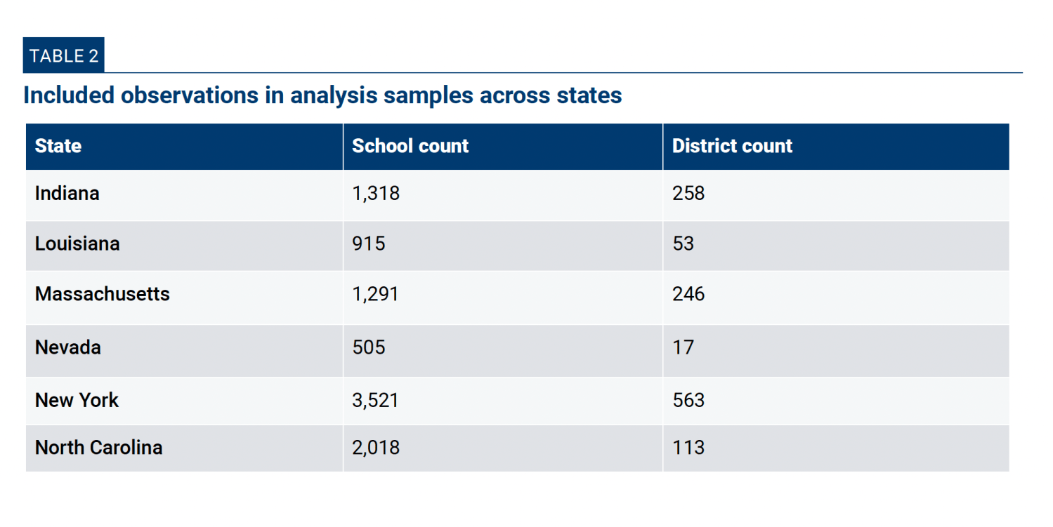
The final observation counts for each of the state analysis samples appear in Appendix Table 2.
Poverty Measures
The proportion of students eligible for the federal free or reduced-price lunch program (FRPL) is the primary measure we use to proxy for poverty at the school level. Eligibility for the program can be determined by direct certification (based on eligibility for federal welfare programs) or through individual applications where family income must be below 130% (for free) or 185% (for reduced) of the federal poverty income level.
Chapter 1
We use student eligibility for FRPL, where available, and student direct certification counts where FRPL data are unavailable. In the vast majority of cases, one measure or the other (or both) is reported for all schools in a district. There are exceptions, where schools within the same district have different data available. In these cases, we only include schools that report the same measure as other schools in their district. This is necessary because student poverty measured through direct certification yields a smaller percentage of estimated disadvantaged students than student poverty measured through FRPL eligibility (even for the same group of students). We take this approach to maintain a uniform measure for within-district calculations.
Chapter 2
In our analysis sample for Chapter 2, Indiana and Massachusetts reported their school poverty as direct certification numbers, while Louisiana, New York, and North Carolina reported their numbers based on applications and eligibility for FRPL. Nevada reported both metrics, and we chose to use direct certification numbers for this chapter’s analysis as it showed greater variation across and within districts.
Inequality calculations
In both chapters we use the weighted average of money spent on economically disadvantaged students and economically advantaged students to determine inequalities. The formula for the weighted average calculation is:
1)

2)
 Essentially, spending on either student group is a weighted average of school-level per-pupil spending and the NCES wage index, which is defined at the district level and is intended to make cost-of-living differences comparable across regions. Since we are using within-district ratios in Chapter 1 and the wage index does not vary within a district, we do not use it in that portion of the analysis.
The numerator of ??,? represents the total count of FRPL-eligible (economically disadvantaged) or non-FRPL students (g) at each school (s), while the denominator sums the same value across all schools within a district (d) or state. Intuitively, the weight represents the number of FRPL or non-FRPL students in the school as a share of the total number in the same groups across the entire district or state.
Taken together, the calculations represent the share of spending allocated to FRPL and non-FRPL students across the analysis unit. These inequality figures will be accurate to the extent that reported spending in the NERD$ data is accurate, and with the assumption that per-pupil spending does not systematically vary across groups within schools. We discuss these implications in each chapter.
The same formulas can be computed separately at the district or state level; the only difference between the two models is the denominator in the weight used in the formula. When reporting spending inequalities within districts across the state, district-level values are combined using a weighted average based on district total enrollment.
Chapter 1
Funding inequalities are calculated with the following formula:
3)
 The funding gap is determined by the ratio between spending on economically disadvantaged (FRPL) and economically advantaged (non-FRPL) students within a district—based on allocations to the schools in which they are enrolled. A value greater than 1 indicates that more is spent on FRPL students relative to non-FRPL students and a value smaller than 1 indicates the opposite. Note, for interpretation, that a district that spends twice as much on FRPL students will have a ratio of 2 while a district that spends half as much on FRPL students will have a ratio of 0.5 (i.e., not equidistant from 1).
Chapter 2
Funding inequalities are calculated with the following formula:
4)
 The spending inequality formulas can also be modified to explore differences in staffing variables. This is done by simply substituting the desired staffing measure in place of per-pupil spending in equation 1. One of our variables related to access to teachers is an indicator of a negative condition (percentage of the teacher workforce who are novices). For this measure only, we multiply the calculated result by -1 so the interpretation of the result is consistent with all other inequality measures presented. Thus, across all inequality measures, positive values indicate regressive outcomes and negative values indicate progressive outcomes.
Regression models
Chapter 1
We estimate regression models using both the main national sample and the smaller school board sample with the spending ratio measure as our dependent variable. The specifications for the regressions are detailed in the tables reported in the chapter of the main report.
Chapter 2
We run regression models using a series of staffing variables as our dependent variables. The regression equation is:
5)
 The three staffing variables as dependent variables are the share of novice teachers, staffing ratios for FTE teachers per 100 students, and staffing ratios of FTE teacher aides and other instructional support staff per 100 students. All staffing variables are measured at the school level and the regression models are run as a series of separate models. The explanatory variables are the same in each model and include the share of FRPL students in the school (????%?) with the share of economically disadvantaged students proxied by the share of either FRPL-eligible or direct-certified students), the log of student enrollment, and indicator variables on school level (middle schools, high schools, and other grade arrangements—elementary schools are the omitted category) represented as ??.
We are primarily interested in the point estimate ?1^ which shows how each dependent variable is related to the share of economically disadvantaged students in the school, conditioned on the other covariates.
Authors


The Brookings Institution is committed to quality, independence, and impact.
We are supported by a diverse array of funders. In line with our values and policies, each Brookings publication represents the sole views of its author(s).