
This Hamilton Project policy memo provides thirteen economic facts on the growth of income inequality and its relationship to social mobility in America; on the growing divide in educational opportunities and outcomes for high- and low-income students; and on the pivotal role education can play in increasing the ability of low-income Americans to move up the income ladder.
Read the full introduction »
It is well known that the income divide in the United States has increased substantially over the last few decades, a trend that is particularly true for families with children. In fact, according to Census Bureau data, more than one-third of children today are raised in families with lower incomes than comparable children thirty-five years ago. This sustained erosion of income among such a broad group of children is without precedent in recent American history. Over the same period, children living in the highest 5 percent of the family-income distribution have seen their families’ incomes double.
What is less well known, however, is that mounting evidence hints that the forces behind these divergent experiences are threatening the upward mobility of the youngest Americans, and that inequality of income for one generation may mean inequality of opportunity for the next. It is too early to say for certain whether the rise in income inequality over the past few decades has caused a fall in social mobility of the poor and those in the middle class—the first generation of Americans to grow up under this inequality is, on average, in high school—but the early signs are troubling.
Investments in education and skills, which are factors that increasingly determine outcomes in the job market, are becoming more stratified by family income. As income inequality has increased, wealthier parents are able to invest more in their children’s education and enrichment, increasing the already sizable difference in investment from those at the other end of the earnings distribution. This disparity has real and measurable consequences for the current generation of American children. Although cognitive tests of ability show little difference between children of high- and low-income parents in the first years of their lives, large and persistent differences start emerging before kindergarten. Among older children, evidence suggests that the gap between high- and low-income primary and secondary-school students has increased by almost 40 percent over the past thirty years.
These differences persist and widen into young adulthood and beyond. Just as the gap in K–12 test scores between high and low-income students is growing, the difference in college graduation rates between the rich and the poor is also growing. Although the college graduation rate among the poorest households increased by about 4 percentage points between those born in the early 1960s and those born in the early 1980s, over this same period, the graduation rate increased by almost 20 percentage points for the wealthiest households.
Given how important education and, in particular, a college degree are in the labor market, these trends give rise to concerns that last generation’s inequities will be perpetuated into the next generation and opportunities for upward social mobility will be diminished. The emphasis that American society places on upward mobility makes this alarming in and of itself. In addition, low levels of social mobility may ultimately shift public support toward policies to address such inequities, instead of toward policies intended to promote economic growth.
While the urgency of finding solutions to this challenge requires rethinking a broad range of social and economic policies, we believe that any successful approach will necessitate increasing the skills and human capital of Americans. Decades of research demonstrate that policies that improve the quality of and expand access to early-childhood, K–12, and higher education can be effective at ameliorating these stark differences in economic opportunities across households.
Indeed, making it easier and more affordable for low-income students to attend college has long been a vehicle for upward mobility. Over the past fifty years, policies that have increased access to higher education, from the GI Bill to student aid, have not only helped lift thousands of Americans into the middle class and beyond, but also have boosted the productivity, innovation, and resources of the American economy.
Fortunately, researchers are making rapid progress in identifying new approaches that complement or improve on long-standing federal aid programs to boost college attendance and completion among lower-income students. These new interventions, which include high school and college mentoring, targeted informational interventions, and behavioral approaches to nudge students into better outcomes, could form the basis of important new policies that aim to steer more students toward college.
A founding principle of The Hamilton Project’s economic strategy is that long-term prosperity is best achieved by fostering economic growth and broad participation in that growth. This principle is particularly relevant in the context of social mobility, wherein broad participation in growth can contribute to further growth by providing families with the ability to invest in their children and communities, optimism that their hard work and efforts will lead to success for them and their children, and openness to innovation and change that lead to new sources of economic growth.
In this spirit, we offer our “Thirteen Economic Facts about Social Mobility and the Role of Education.” In chapter 1, we examine the very different changes in income between American families at opposite ends of the income distribution over the last thirty-five years and the seemingly dominant role that a child’s family income plays in determining his or her future economic outcomes. In chapter 2, we provide evidence on the growing divide in the United States in educational opportunities and outcomes based on family income. In chapter 3, we explore the great potential of education to increase upward mobility for all Americans, with a special focus on what we know about how to increase college attendance and completion for low-income students.
Chapter 1: Inequality Is Rising against a Background of Low Social Mobility
Central to the American ethos is the notion that it is possible to start out poor and become more prosperous: that hard work—not simply the circumstances you were born into—offers real prospects for success. But there is a growing gap between families at the top and bottom of the income distribution, raising concerns about the ability of today’s disadvantaged to work their way up the economic ladder.
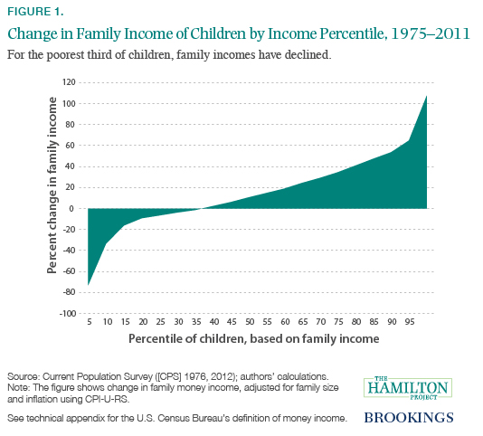
1. Family incomes have declined for a third of American children over the past few decades.
Although family income has increased by an average of 37 percent between 1975 and 2011, family incomes have actually declined for the poorest third of children.
Figure 1 illustrates the diverging fortunes of children based on their family’s income, as measured by the U.S. Census Bureau. Children in families at the top of the income distribution have experienced sizable gains in their families’ incomes and resources since 1975. Children living in the top 5 percent of families, for instance, have seen a doubling of their families’ incomes. But such gains have been more modest for children in the middle of the distribution, and children living in lower-income families have experienced outright declines in incomes. In fact, in 2011 the bottom 35 percent of children lived in families with lower reported incomes than comparable children thirty-six years earlier.
Because of widening disparities in the earnings of their parents and changes in family structure—particularly the increase in single-parent families—the family resources available to lesswell- off children are falling behind those available to their higher-income peers.
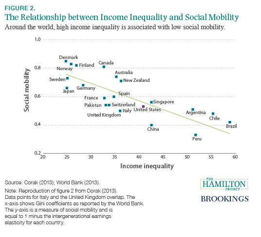
2. Countries with high income inequality have low social mobility.
Many are concerned that rising income inequality will lead to declining social mobility. Figure 2, recently coined “The Great Gatsby Curve,” takes data from several countries at a single point in time to show the relationship between inequality and immobility. Inequality is measured using Gini coefficients, a common metric that economists use to determine how much of a nation’s income is concentrated among the wealthy; social mobility is measured using intergenerational earnings elasticity, an indicator of how much children’s future earnings depend on the earnings of their parents.
Although, as the figure shows, higher levels of inequality are positively correlated with reductions in social mobility, we do not know whether inequality causes reductions in mobility. After all, there are many important factors that vary between countries that might explain this relationship. Nonetheless, figure 2 represents a provocative observation with potentially important policy ramifications.
What figure 2 makes clear is that, although most people think of the United States as the land of opportunity—where hard workers from any background can prosper—the reality is far less encouraging. In fact, in terms of both income inequality and social mobility, the United States is in the middle of the pack when compared to other nations, most of which are democratic countries with market economies.
3. Upward social mobility is limited in the United States.
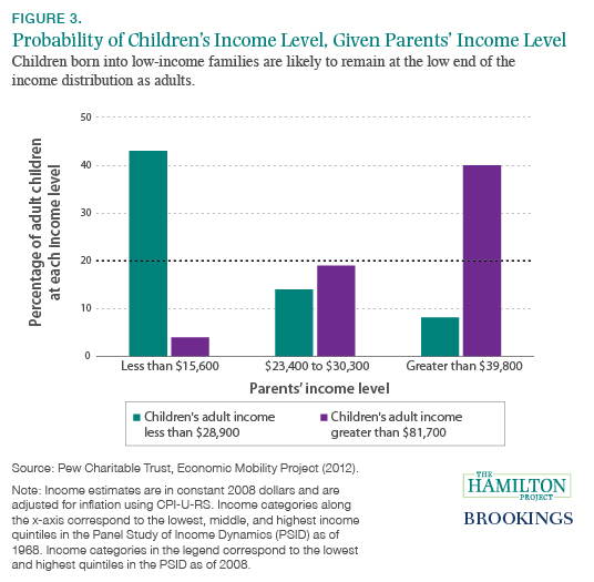
While social mobility and economic opportunity are important aspects of the American ethos, the data suggest they are more myth than reality. In fact, a child’s family income plays a dominant role in determining his or her future income, and those who start out poor are likely to remain poor.
Figure 3 shows the chances that a child’s future earnings will place him in the lowest quintile (that is, the bottom 20 percent of the earnings distribution, shown by the green bars) or the highest quintile (that is, the top 20 percent of the distribution, purple bars) depending on where his parents fell in the distribution (from left to right on the figure, the lowest, middle, and highest quintiles). In a completely mobile society, all children would have the same likelihood of ending up in any part of the income distribution; in this case, all bars on figure 3 would be at 20 percent, denoted by the bold line.
The figure demonstrates that children of well-off families are disproportionately likely to stay well off and children of poor families are very likely to remain poor. For example, a child born to parents with income in the lowest quintile is more than ten times more likely to end up in the lowest quintile than the highest as an adult (43 percent versus 4 percent). And, a child born to parents in the highest quintile is five times more likely to end up in the highest quintile than the lowest (40 percent versus 8 percent). These results run counter to the historic vision of the United States as a land of equal opportunity.
Chapter 2: The United States Is Experiencing a Growing Divide in Educational Investments and Outcomes Based on Family Income
Although children of high- and low-income families are born with similar abilities, high-income parents are increasingly investing more in their children. As a result, the gap between high- and low-income students in K–12 test scores, college attendance and completion, and graduation rates is growing.
4. The children of high- and low-income families are born with similar abilities but different opportunities.
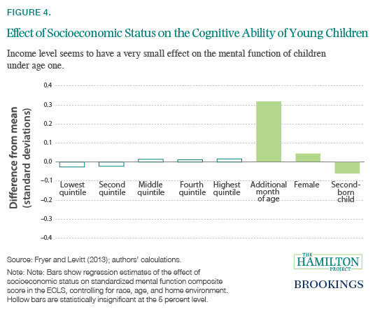
In examining the opportunity gap between high- and low-income children, it is important to begin at the beginning— birth. The evidence suggests that children of high- and low-income families start out with similar abilities but rapidly diverge in outcomes.
At the earliest ages, there is almost no difference in cognitive ability between high- and low-income individuals. Figure 4 shows the impact of a family’s socioeconomic status—a combination of income, education, and occupation—on the cognitive ability of infants between eight and twelve months of age, as measured in the Early Childhood Longitudinal Survey. Although it is obviously difficult to measure the cognitive ability of infants, this ECLS metric has been shown to be modestly predictive of IQ at age five (Fryer and Levitt 2013).
Controlling for age, number of siblings, race, and other environmental factors, the effects of socioeconomic status are small and statistically insignificant. A child born into a family in the highest socioeconomic quintile, for example, can expect to score only 0.02 standard deviations higher on a test of cognitive ability than an average child, while one born into a family in the lowest socioeconomic quintile can expect to score about 0.03 standard deviations lower—hardly a measurable difference and statistically insignificant. By contrast, other factors, such as age, gender, and birth order, have a greater impact on abilities at the earliest stages of life.
Despite similar starting points, by age four, children in the highest income quintile score, on average, in the 69th percentile on tests of literacy and mathematics, while children in the lowest income quintile score in the 34th and 32nd percentile, respectively (Waldfogel and Washbrook 2011). Research suggests that these differences arise largely due to factors related to a child’s home environment and family’s socioeconomic status (Fryer and Levitt 2004).
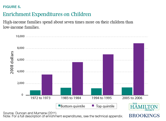
5. There is a widening gap between the investments that high- and low-income families make in their children.
Although we may all enter the world on similar footing, the deck is stacked against children born into low-income households. One significant consequence of growing income inequality is that, by historical standards, high-income households are spending much more on their children’s education than low-income households. Figure 5 shows enrichment expenditures—SAT prep, private tutors, computers, music lessons, and the like—by income level.
Over the past four decades, families at the top of the income ladder have increased spending in these areas dramatically, from just over $3,500 to nearly $9,000 per child per year (in constant 2008 dollars). By comparison, those at the bottom of the income distribution have increased their spending since the early 1970s from less than $850 to about $1,300. The difference is still stark: high-income families have gone from spending slightly more than four times as much as low-income families to nearly seven times more.
Parents of higher socioeconomic status invest not only more money in their children, but more time as well. On average, mothers with a college degree spend 4.5 more hours each week engaging with their children than mothers with only a high school diploma or less (Guryan, Hurst, and Kearney 2008). This means that, among other things, by age three, children of parents who are professionals have vocabularies that are 50 percent larger than those of children from working-class families, and 100 percent larger than those of children whose families receive welfare, disparities that some researchers ascribe to differences in how much parents engage and speak with their children. By the time they are three, children born to parents who are professionals have heard about 30 million more words than children born to parents who receive welfare (Hart and Risley 1995).
6. The achievement gap between high- and low-income students has increased.
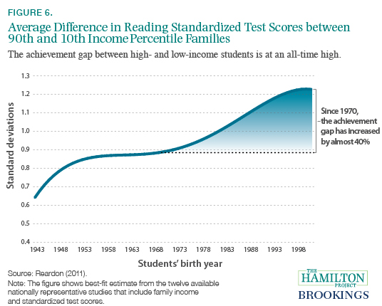
Disparities in what parents can invest in their children—whether time or money—appear to have important consequences for children’s success in school. While many factors play a role in shaping scholastic achievement, family income is one of the most persistent and significant. In fact, the income achievement gap—the role that wealth plays in educational attainment—has been increasing over the past five decades. By comparing test results of children from families at the 90th income percentile to those of children from families at the 10th percentile, researchers have found that the gap has grown by about 40 percent over the past thirty years (Reardon 2011).
Figure 6 shows that the income achievement gap as estimated for students born in 2001 is over 1.2 standard deviations. To put this in perspective, according to the National Assessment of Educational Progress, an average student advances between 1.2 and 1.5 standard deviations between fourth and eighth grade. The achievement gap between high- and low-income students, then, is on par with the gap between eighth graders and fourth graders.
This growing test-score gap mirrors the diverging parental investments of high- and low-income families (figure 5). As with parental investment, the test scores of low-income students have shown modest gains over the past few decades, while those of high-income students have shown large increases. The gap between high- and low-income students, therefore, is not an instance of the poor doing worse while the wealthy are doing better; rather, it is that students from wealthier families are pulling away from their lower-income peers.
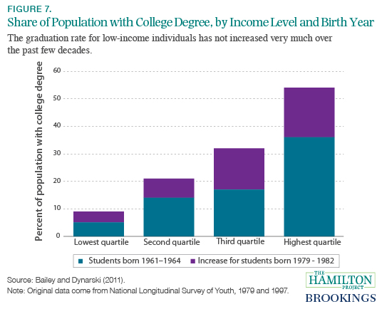
7. College graduation rates have increased sharply for wealthy students but stagnated for low-income students.
College graduation rates have increased dramatically over the past few decades, but most of these increases have been achieved by high-income Americans. Figure 7 shows the change in graduation rates for individuals born between 1961 and 1964 and those born between 1979 and 1982. The graduation rates are reported separately for children in each quartile of the income distribution.
In every income quartile, the proportion graduating from college increased, but the size of that increase varied considerably. While the highest income quartile saw an 18 percentage-point increase in the graduation rate between these birth cohorts, the lowest income quartile saw only a 4 percentage-point increase.
This graduation-rate gap may have important implications for social mobility and inequality. Given the importance of a college degree in today’s labor market, rising disparities in college completion portend rising disparities in outcomes in the future.
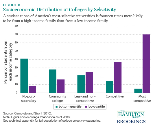
8. High-income families dominate enrollment at America’s selective colleges.
The gap between high- and low-income groups in college outcomes extends beyond college graduation rates. Students from higher-income families also apply to and enroll in moreselective colleges. Figure 8 reports the percent of students at more- and less-selective schools that come from families in the top and bottom quartiles of the socioeconomic status distribution (a combination of parental income, education, and occupation).
The figure demonstrates that the most-competitive colleges are attended almost entirely by students from higher–socioeconomic status households. Indeed, the more competitive the institution, the greater the percentage of the student body that comes from the top quartile, and the smaller the percentage from the bottom quartile. At institutions ranked as “most competitive”—those with more-selective admissions and that require high grades and SAT scores— the wealthiest students out-populate the poorest students by a margin of fourteen to one (Carnevale and Strohl 2010). By contrast, at institutions ranked as “less-competitive” and “noncompetitive,” the lowest–socioeconomic status students are over-represented.
Chapter 3: Education Can Play a Pivotal Role in Improving Social Mobility
Promoting increased social mobility requires reexamining a wide range of economic, health, social, and education policies. Higher education has always been a key way for poor Americans to find opportunities to transform their economic circumstances. In a time of rising inequality and low social mobility, improving the quality of and access to education has the potential to increase equality of opportunity for all Americans.
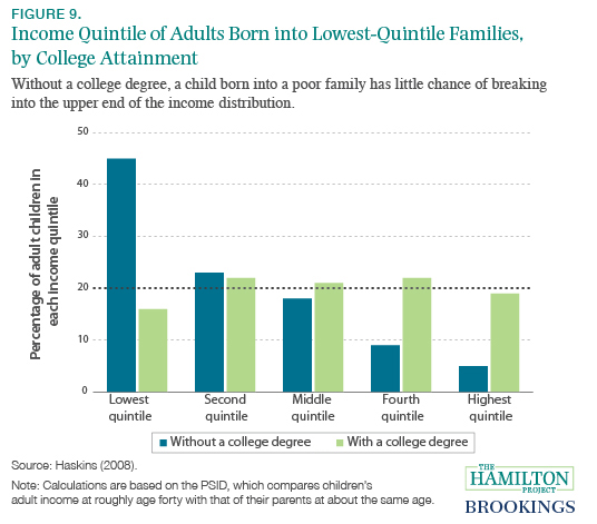
9. A college degree can be a ticket out of poverty.
The earnings of college graduates are much higher than for nongraduates, and that is especially true among people born into low-income families. Figure 9 shows the earnings outcomes for individuals born into the lowest quintile of the income distribution, depending on whether they earned a college degree. In a perfectly mobile society, an individual would have an equal chance of ending up in any of the five quintiles, and all the bars would be level with the bold line.
As the figure shows, however, without a college degree a child born into a family in the lowest quintile has a 45 percent chance of remaining in that quintile as an adult and only a 5 percent chance of moving into the highest quintile. On the other hand, children born into the lowest quintile who do earn a college degree have only a 16 percent chance of remaining in the lowest quintile and a 19 percent chance of breaking into the top quintile. In other words, a low-income individual without a college degree will very likely remain in the lower part of the earnings distribution, whereas a low-income individual with a college degree could just as easily land in any income quintile—including the highest.
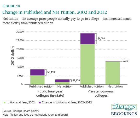
10. The sticker price of college has increased significantly in the past decade, but the actual price for many lower- and middle-income students has not.
In the past decade, increases in the sticker price of attending college have made going to college appear, for some, prohibitively expensive. Published tuition and fees for the 2012–13 academic year are projected to average $26,060 for private four-year institutions, and $8,860 in-state for public four-year institutions (College Board 2012). But before allowing this sticker price to be a deterrent, students must look deeper to learn whether those costs apply to them. Looking at net tuition—the price that the average student actually pays after financial aid—the picture is very different.
Because of increases in federal, state, and college-provided financial aid, not only is average net tuition much lower than average published tuition, but it has also increased at a much lower rate than published tuition in the past ten years. As seen in figure 10, net in-state tuition and fees at public four-year colleges have only increased by an average of $1,420 since 2002, which is less than half of the increase in the published rate. Although published tuition at private four-year colleges has increased by an average of $6,090 since 2002, net tuition has only increased by $230. In fact, the projected average net tuition at private four-year colleges for the academic year 2012–13 is 3.7 percent lower than the average net tuition in 2007–08 and lower than all five academic years between 2004–05 and 2008–09 (College Board 2012).
For many households, high costs of tuition are a burden. Once families and students have a sense of what financial aid they are eligible for, they can get a more accurate idea of the actual price tag for tuition. For each student, the net cost is the important consideration when making educational decisions.
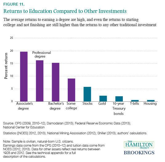
11. Few investments yield as high a return as a college degree.
Obtaining a college degree can significantly boost one’s income. Over the past three years, individuals between the ages of thirty and fifty who graduated from high school but did not attend college could expect to earn less than $30,000 per year. Those whose highest level of educational attainment was a bachelor’s degree earned just under $60,000 per year, and those with an advanced degree earned over $80,000.
But even individuals who attend college and do not obtain a degree still see an increase in their annual earnings. Those who leave college before receiving a credential or degree earn about $7,000 per year more than those with only a high school diploma, and individuals holding an associate’s degree earn over $10,000 more.
Higher education is one of the best investments an individual can make. As shown in figure 11, the returns to earning an associate’s, professional, or bachelor’s degree exceed 15 percent, and even the average return to attending some college for those who do not earn a degree is 9 percent. In comparison, the average return to an investment in the stock market is a little over 5 percent; gold, ten-year Treasury bonds, T-bills, and housing are 3 percent or less.
Although the return to an associate’s degree really stands out, this high return partially reflects the lower cost of an associate’s degree rather than a major boost to long-run earnings. Over a lifetime, the earnings of an associate’s degree recipient are roughly $170,000 higher than those of a high school graduate, while the earnings of a bachelor’s degree holder are $570,000 more than those of a high school graduate.
While it is likely that college graduates have different aptitudes and ambitions that might affect earnings and thus the resulting economic returns, a large body of academic research suggests there is a strong causal relationship between increases in education and increases in earnings (Card 2001).
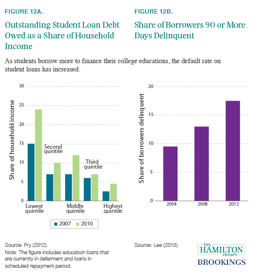
12. Students are borrowing more to attend college—and defaulting more frequently on their loans.
Over the past decade, the volume and frequency of student loans have increased significantly. The share of twenty-five-year-olds with student debt has risen by about 15 percentage points since 2004, and the amount of student debt incurred by those under the age of thirty has more than doubled (Lee 2013).
Despite these increases, the majority of students appear to borrow prudently. About 90 percent have loan balances less than $50,000, and 40 percent have balances under $10,000 (Fry 2012). Given that a college graduate can expect to earn, on average, about $30,000 more per year than a high school graduate over the course of his or her life, the returns to college appear to warrant the cost of student loans for most students.
Still, recent trends in student loans raise questions and concerns that merit further investigation. For one, it is unclear why student debt is increasing at its current trajectory. Neither college enrollment nor net college tuition has risen dramatically enough over the past decade to explain the rapid upsurge. Second, even though most students have a relatively low total loan balance, the default rate has increased significantly over the past decade: the share of those more than ninety days delinquent rose from under 10 percent in 2004 to about 18 percent in 2012 (figure 12b). While the returns to investments in college remain high, it will be important for policymakers to better understand why debt and delinquency rates have increased over the past decade.
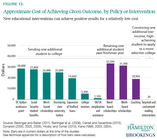
13. New low-cost interventions can encourage more low-income students to attend, remain enrolled in, and increase economic diversity at even top colleges.
To promote social mobility, enabling more low- and middle-income students to pay for college with federal grants is one of the most important goals that policymakers can pursue. For the past several decades, the main tools for achieving this goal have been Pell grants, Stafford loans, or merit-based aid such as the state of Georgia’s HOPE Scholarship. Researchers estimate that, depending on the exact program, the effect of $1,000 of college aid is an increase of 3 to 6 percentage points in college enrollment (Deming and Dynarski 2009). As figure 13 shows, this translates into a total cost of between $20,000 and $30,000 to send one additional student to college through these aid programs. To put this in context, the average difference in earnings between a college graduate and a high school graduate is almost $30,000 per year, so these programs are likely to be beneficial on net.
Figure 13 also reports on new, low-cost interventions that can complement federal and state aid programs to send more kids to college and to better schools, and to convince them to stay in college once they get there. One study finds that simplifying and assisting low-income students in the financial aid application process increases college enrollment by about 8 percentage points, and costs less than $100 per student (Bettinger et al. 2009). And, on a per student basis, employing mentors to coach students on the value of staying in college beyond their freshman years is $10,000 less expensive than need- or merit-based scholarships (Bettinger and Baker 2011).
Another study found that mailing high-achieving, low-income students personalized information on their college options nudged those students to apply to better schools. At a cost of only $6 per student contacted, this intervention increased low-income students’ applications to selective schools by more than 30 percentage points (Hoxby and Turner 2013).
Related Content


Related Books

The Brookings Institution is committed to quality, independence, and impact.
We are supported by a diverse array of funders. In line with our values and policies, each Brookings publication represents the sole views of its author(s).