

Most economists and policymakers know that people who complete a college degree tend to earn more than people who have not attended college. Yet they often overlook the fact that these benefits extend beyond individual workers. The college earnings advantage also leads to greater economic activity, fueling prosperity at the regional and national levels.
With these benefits in mind, this brief finds the following:
The average bachelor’s degree holder contributes $278,000 more to local economies than the average high school graduate through direct spending over the course of his or her lifetime; an associate degree holder contributes $81,000 more than a high school graduate.
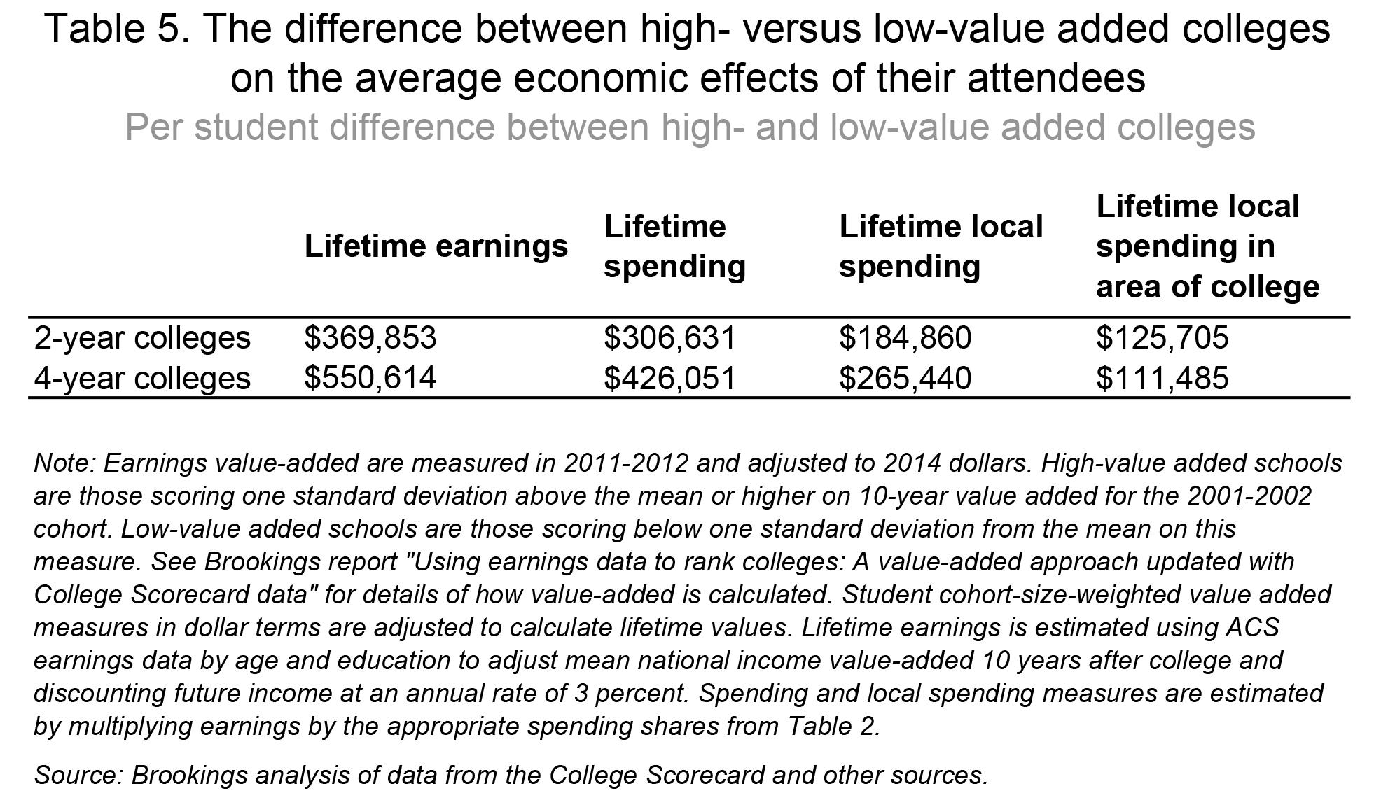
The quality of colleges greatly affects the size of these benefits. High value-added four-year colleges contribute $265,000 more per student to local economies than low-value added four-year colleges. The contribution is $184,000 for high value-added two-year colleges.
Sixty-eight percent of alumni from two-year colleges remain in the area of their college after attending, compared to 42 percent of alumni from four-year colleges. High-value added colleges are no more or less likely to retain students in their metropolitan area.
State and local governments, as well as their taxpayers, have a very strong incentive to boost college attendance and completion, especially at higher quality institutions. Risk-sharing of federal student loans—based on value-added principles—is one promising approach to promoting greater economic returns for students and taxpayers.
Measuring the effect of education on economic growth
Many economists have noted the high correlation between regional economic growth and higher educational attainment, which can be observed in the recent rise of metropolitan areas like San Jose, Austin, Washington D.C., and Boulder, Colo.. Ed Glaeser’s work has explored this relationship in great depth. But teasing out precisely how much GDP growth can be attributed to education is very difficult using standard statistical methods. Highly educated places are richer in part because more high earning individuals reside there or have moved there, but it is likely that other growth-inducing factors drew them to the area—like the presence of innovative companies, favorable state or local laws, or geographic attributes.
To get at the issue, I try a different approach based on accounting rather than regression analysis. We know from survey data how much people of different income and education levels spend on various goods and services. If education is the cause of higher incomes, and higher incomes drive higher spending, then the causal effect of college education on consumption is approximately the difference in consumption between college attendees and non-attendees.
As it happens, there is overwhelming evidence—from twin studies and from quasi-experiments—that education causes higher earnings and the causal effect of college on earnings is close to the average difference in earnings between college educated and high school educated workers. To the latter point, even though wealthier individuals save a higher percentage of their income, they also spend more than less wealthy individuals.
One limitation of this approach is that consumption is only one contributor to economic activity. Innovation, likely enhanced by education, can cause growth in real incomes by lowering the price of goods and services, but these effects are unlikely to concentrate in the location of production, since the benefits will go to consumers around the world, depending on the product. One could also imagine highly skilled workers affecting growth by contributing to the productivity of their colleagues, as economist Enrico Moretti has argued. For these reasons, the calculations below should be considered a conservative estimate of how college education affects growth.
Local goods and services
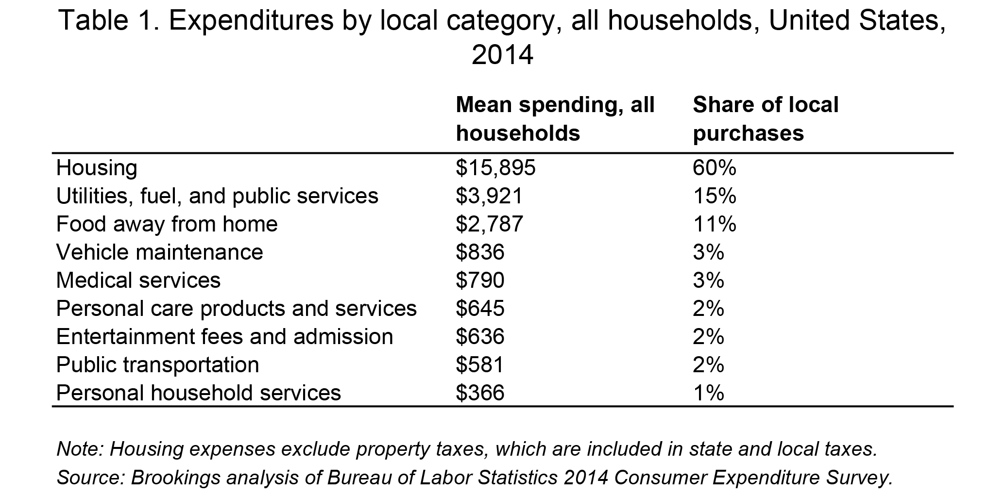
Consumption data by education and income for 2014 are available through the Bureau of Labor Statistics’ Consumer Expenditure Survey. I categorize certain expenditures as “local,” if the value is mostly created by local businesses and the rest as national or international (Table 1).
This admittedly requires subjective judgment. A guiding principle is that most goods purchases should not be thought of as local, given that most merchandise is produced outside the local area where it is eventually consumed, but most services are local. On the services side, I exclude education, health insurance, and life insurance services and a few others that are grouped with the purchase of goods.
Overall, I estimate that 40 percent of pre-tax income and 49 percent of spending goes toward local goods and services, which amounts to $3.4 trillion. The largest source of local spending goes to the housing market. In reality, not all housing spending is local, since some owners live outside the metropolitan area, but the majority of value stays within the region. Data are hard to come by, but a Census Bureau survey from 1995 shows that the vast majority of owners of multi-family buildings at least occasionally visit the premises, suggesting residential proximity. Owner-occupied home purchases and the local services that support those transactions are almost entirely local. Other big local expenditures include utilities and restaurants or bars.
Consumption, taxes, and education
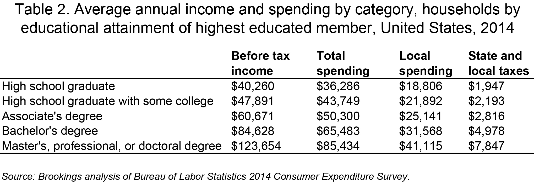
Highly educated households spend much more on the local economy than their less educated peers. It is not that highly educated households concentrate a higher share of their spending on local goods and services, but their gross spending power is so much greater that graduate degree earners spend more than twice as much on local goods and services as high school graduates. Tax expenditure flows to state and local governments, which are largely based on property, sales, and income taxes, rise sharply as household education increases.
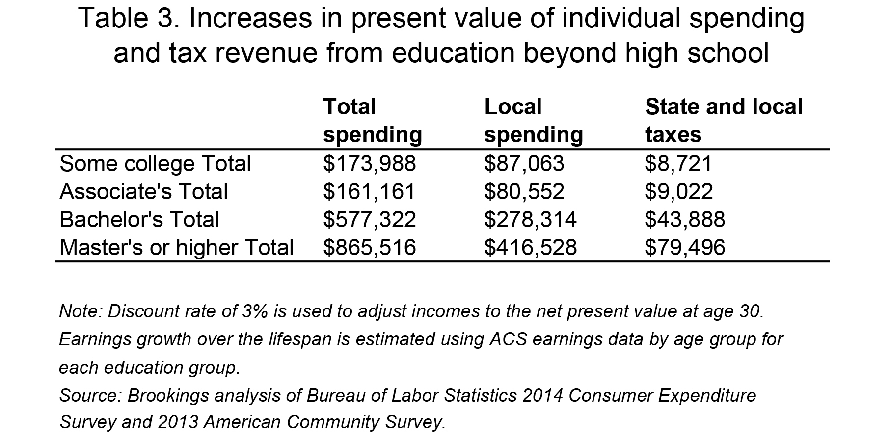
Over the course of a lifetime, these annual differences in consumption and taxes add up to very large amounts. To estimate lifetime spending, I collect earnings data for those in the labor force and aged 25 to 64 by age and education from the 2013 American Community Survey (ACS) using the Integrated Public Use Micro Data Series (IPUMS). I use the average share of income consumed by education and hold that constant over the lifetime, but allow income to rise and fall by age separately for each education group. Future spending flows are then discounted using a 3 percent interest rate, which affectively shrinks the value of future income to what it would be worth at age 30.
After making these calculations, the average bachelor’s degree holder will spend an estimated $278,000 more on local goods and services than the average high school graduate over a lifetime. Local and state taxes will be $44,000 higher. Even an associate degree holder will spend $81,000 more on average over his or her lifetime, including an additional $9,000 in state and local taxes.
The state and local tax estimates here should be regarded as incomplete for a number of reasons. These estimates do not consider the reduction in government spending as a result of education (e.g. lower health bills, welfare, or crime costs); More broadly, the estimates do not account for multiplier effects, that for every additional dollar spent, some fraction will be spent again by the next person. For these reasons, it is very likely that a policy that resulted in one extra associate degree holder at an upfront cost of more than $9,000 to state and local taxpayers would still pay for itself in the long run. The City University of New York has experimented with one such policy, which was able to double graduation rates while spending an additional $5,000 per student per year. After including some of these other considerations, scholars at Columbia University determined that the CUNY ASAP program generates $146,000 in lifetime benefits to taxpayers.
For any given place, the estimates of state and local benefits are also affected by whether or not alumni remain in the area. To the extent that the area is a net loser in the migration of college attendees, local and state benefits will dissipate accordingly and be captured by the areas where the alumni relocate. Using data from LinkedIn alumni profiles, my colleague Sid Kulkarni and I were able to calculate the percentage of alumni from roughly 1700 colleges who work in the same metropolitan area as their college. Overall, 68 percent of two-year attendees remain in the same area after graduating, compared to 42 percent of four-year attendees. I consider these shares below in estimating how the quality of colleges affects the local benefits to a particular place.
How college quality affects earnings
The above calculations assume all colleges are of the same quality, but alumni earnings differ dramatically by institution, even after accounting for student family income and other demographic characteristics. My recent research on the value-added of specific colleges reports these data. Thus, enhancing the quality of colleges with respect to earnings is another important way to increase the local economic benefits of colleges.
To quantify quality, I first distinguish high- and low-value added colleges based on those that are one standard deviation above and one standard deviation below the mean, respectively, using my recent research. Then I calculate the average dollar amount added to alumni salaries for high- and low-value added schools on a per student basis. An alternative approach would simply distinguish colleges by the earnings of their alumni, and for local tax accounting that is more relevant. However, from a national public policy perspective differentiating whether a college benefits an area because it is drawing in top students from other areas (thus depriving those areas of high-potential earners) or generating higher than expected benefits for less advantaged students as well as the affluent is more valuable.
The amount colleges add to the value of alumni earnings can be applied to mean earnings from the Consumer Expenditure Survey to get a sense of what earnings look like in these two groups compared to the mean (Table 4).1 If the average college student had attended a high-value added four-year college, he or she would have earned $97,000 instead of the mean of $85,000, and going to a low-value added college would result in just $78,000.2
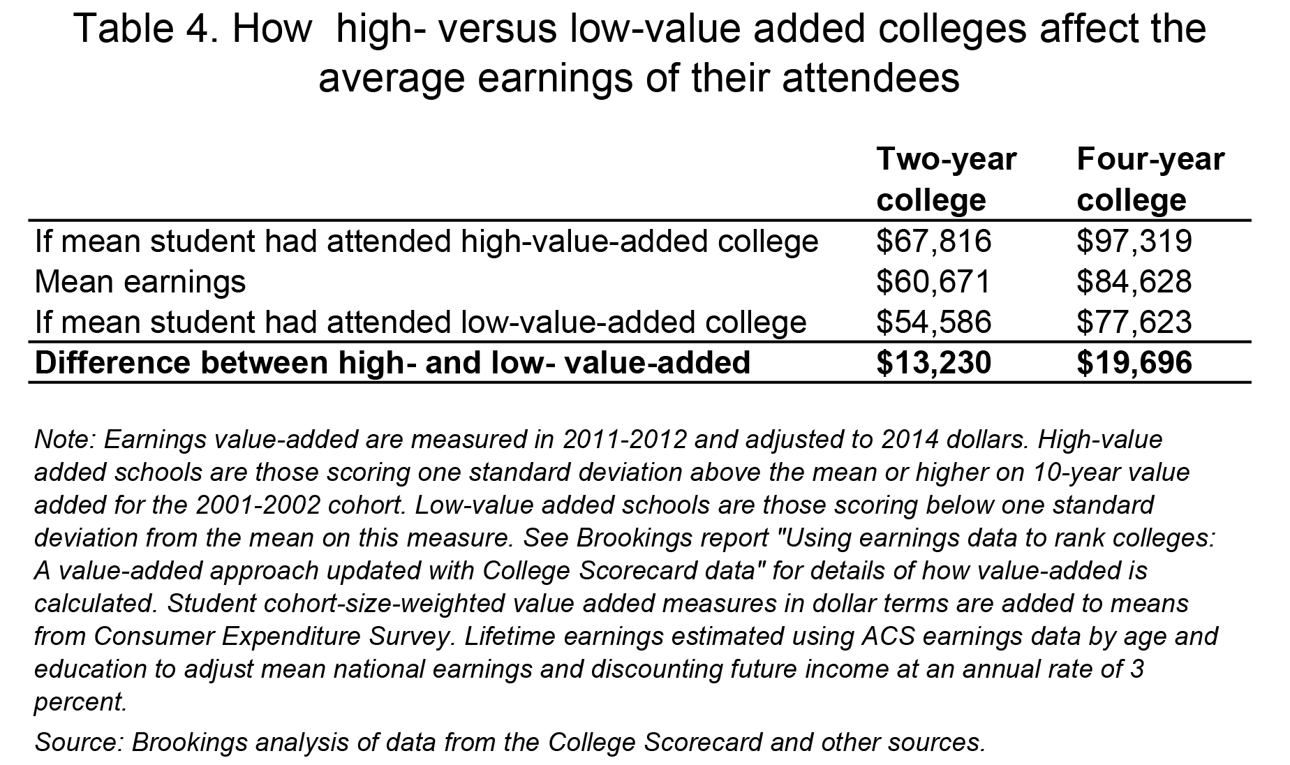
Assuming the earnings differences after 10 years of attendance hold up for the rest of the attendees’ working lives, a net present value estimate can be calculated for the lifetime spending differences in attending high versus low value-added colleges, after adjusting incomes by the national savings rates for the appropriate level of education. For four-year schools, the spending difference amounts to $426,000, and it is $307,000 for two-year colleges. Roughly half of that spending will go toward local economies. Multiplying local spending by the settlement rate—the share of alumni remaining in the area of the college—reduces the effect but still generates $111,000 for four-year colleges and an even higher total of $126,000 for two-year colleges. These estimates imply that states and local economies with high value-added quality colleges enjoy massive economic and tax benefits.
It turns out that the benefits of higher-value added colleges do not come with higher costs. In fact, average tuition is almost $2,000 less at high value-added four-year colleges than it is at low value-added colleges. Tuition is also slightly less at high value-added two-year colleges.
Furthermore, one might be worried that students from higher-value added colleges would be more likely to leave the area, but I find that there is no significant correlation between a college’s value-added score and the percentage of students who remain in the metropolitan area after attending.
Alumni from high-earning schools vary greatly in their propensity to stay in an area. Among four-year colleges, schools like Harvard and Duke, as well as technically focused schools like Rose-Hulman Institute of Technology in Indiana and Rensselaer Polytechnic Institute near Albany generate enormous value for these students, but less than one quarter of alumni remain in the area. On the other hand, 43 percent of Stanford alumni work around San Jose or San Francisco. Sixty-four percent of graduates from the University of Washington in Seattle stay in the Seattle area, and 57 percent of alumni from the Illinois Institute of Technology work in or around Chicago.
At the metropolitan scale, retention rates differ considerably and are modestly correlated with size and measures of worker productivity. The New York City area exhibits one of the highest retention rates with 70 percent of four-year college attendees remaining in the area. Alumni from high value-added colleges there like Columbia University, the Stevens Institute of Technology, Manhattan Colleges, and the CUNY schools tend to stay. Detroit, Houston, Chicago, San Jose, and Atlanta also retain at least 65 percent of attendees from four-year schools. On the other hand, Boston retains just over half (53 percent), and the Washington D.C. area retains just 44 percent, as do Baltimore and Pittsburgh.
Conclusion and policy implications
While most policy leaders and voters might assume that more education is better for the economy, the empirical relationship between economic growth and a highly educated population has been unclear. This report aims to simplify that relationship by understanding one direct channel through which education boosts the level of economic activity in an area: consumption.
This should by no means be regarded as a comprehensive assessment of the public benefits to the economy of education. I have not attempted to consider how education affects government savings, through channels such as criminal behavior or health. I have also not attempted to estimate the role of education in entrepreneurship and innovation, which is likely very large and valuable. Nonetheless, these estimates provide some sense of a minimum benchmark for how education affects a local economy, and they are non-trivial in magnitude even with these caveats.
This analysis also shows that college quality has major implications for the extent to which higher education boosts economic activity. Thus states and their voters have a very clear incentive to raise the quality of their colleges, with respect to how they affect earnings.
In my previous work, I discussed ways of doing that—through increasing the market value of course content and skills taught; investing in a high quality teaching staff, offering financial aid, and implementing programs that will boost retention and graduation.
As I and others have argued, increasing transparency about student outcomes at particular colleges is one potential way to enhance college quality. With those data, a student could more easily choose to attend a college that results in a high salary. Ideally, the public would also have access to data on the quality of learning at a college, but methodological challenges mean that information is unlikely to be available anytime soon.
Additionally, one could imagine state or federal policies that go further in inducing colleges to prepare their students for at least a modicum of economic success after attendance.
For example, colleges could be forced to pay back the federal government a portion of what has been lent out to their students when those students default on federal loans. This would offset some of the risk to taxpayers, while imposing it on chronically bad-performing colleges. The concept is known as “risk-sharing,” and the idea has gained some traction in the Senate and a thoughtful and more detailed proposal has been put forward by Andrew P. Kelly of the American Enterprise Institute, suggesting the idea has bipartisan support.
In order to avoid punishing colleges that admit the low-income students most likely to default, the portion of defaulted debt owed to the federal government could be adjusted based on observable student characteristics, such that it is higher for the students least likely to default and very low for those most likely to default. In short, each school could receive a predicted default level, using similar methods as my value-added research, but only have to pay back the federal government for the difference between the actual and predicted defaulted amount.
The author would like to thank Brad Hershbein and Alan Berube for very helpful comments on an earlier draft.
1. To do this, I convert the percent of value added to earnings into a dollar amount by multiplying it by median earnings at each college. This accounts for the fact that median earnings are sometimes low in high value-added colleges with very low predicted earnings. I use the median rather than mean because the former is not influenced by extreme outliers in earnings, which are probably more attributable to individual characteristics and not the college itself.
2. If I had used mean value-added measures as percentages and assumed each college had average predicted salary for its type, the earnings differences would have been $107,000 versus $68,000 for four-year colleges and $73,000 versus $49,000 for two-year colleges.
The Brookings Institution is committed to quality, independence, and impact.
We are supported by a diverse array of funders. In line with our values and policies, each Brookings publication represents the sole views of its author(s).