I. Introduction
The recent release of new budget data by the Congressional Budget Office (2017) provides an opportunity to update and reassess the fiscal outlook. As it turns out, the fiscal outlook remains largely unchanged from the projections based on CBO’s (2016a) previous release of budget data in August, 2016.
But no news is not always good news. While deficits are manageable in the short run, the debt-GDP ratio is already high relative to historical norms, and projections indicate that both figures will rise in the future, even under optimistic assumptions. Sustained federal deficits and rising federal debt will crowd out future investment, reduce prospects for economic growth, and impose burdens on future generations.
In 2016, the federal budget deficit was $587 billion, or 3.2 percent of GDP. The debt-GDP ratio stood at 77 percent at the end of the year. Under CBO’s current-law projections, the deficit will decrease over the next few years relative to the economy and then rise gradually to 5.0 percent of GDP by 2027, at which point debt will equal 89 percent of the economy.
We provide “current-policy” projections over the next decade and for longer periods. While current-law projections examine the impact of Congress essentially doing nothing over the projection period, current-policy estimates aim to understand the impact of what might be termed “business-as-usual” assumptions. It is worth emphasizing that what constitutes business as usual seems to be particularly uncertain given the new Administration. Nevertheless, for consistency with prior estimates and in the absence of more appropriate choices, we make similar adjustments to the current-law projections as in our own recent studies. In particular, we let defense spending grow with inflation through 2027 and let non-defense discretionary spending grow at the rate of inflation plus population growth through 2027 (rather than following the caps set forth in previous legislation). Additionally, we assume that all temporary tax cut or tax delay provisions are made permanent.
Under these assumptions, we project that by 2027, the federal budget deficit would rise to 6.1 percent of GDP and the debt-GDP ratio would rise to 96 percent. Looking farther out, we project the debt-GDP ratio would rise to 154 percent by 2047 and to higher levels in subsequent years.
The fiscal gap shows the tax and spending changes needed to bring the debt-GDP ratio to a specified level in a specified year. For example, we find that just to ensure that the debt-GDP ratio in 2047 does not exceed the current level would require a combination of spending cuts and tax increases starting in 2017 of 2.75 percent of GDP. This represents about a 14 percent cut in non-interest spending or a 15 percent increase in taxes relative to current levels. To return the debt-GDP ratio in 2047 to 36 percent, its average in the 50 years preceding the Great Recession in 2007-9, would require spending cuts or tax increases of 4.2 percent of GDP.
While the numbers above are projections, not predictions, they nonetheless constitute the fiscal backdrop against which new tax and spending proposals should be considered.
II. The 10-year budget outlook
A. Assumptions
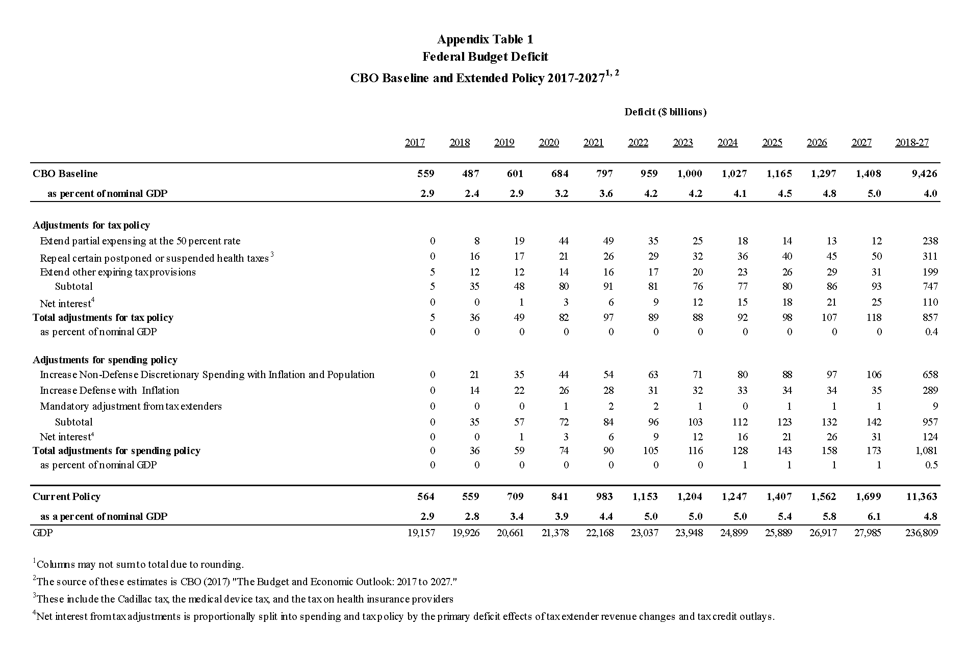
We construct 10-year projections by starting with the CBO’s January 2017 current-law baseline (CBO 2017) and making a series of adjustments. These adjustments are admittedly judgmental. In our view, they provide a better picture of what constitutes current policy than do the CBO current-law projections, which in many instances reflect budget conventions or assumptions that CBO is required to make by law.
On the tax side, we assume that all temporary tax-cut or tax-delay provisions are made permanent. This includes 50 percent expensing of equipment and property for business investment. It also includes the repeal of certain postponed or suspended health care taxes in the Affordable Care Act (ACA), including the medical device excise tax and the tax on high-premium insurance (commonly known as the “Cadillac Tax”). The implementation of these taxes was postponed by two years in the Protecting Americans from Tax Hikes Act of 2015. Additionally, the Administration and Congress have expressed significant interest in permanent repeal of the ACA, and it seems likely that a new health care law will be passed.
On the spending side, CBO sets discretionary spending through 2021 at the levels created by the discretionary spending caps and sequestration procedures (as imposed in the Budget Control Act of 2011 and modified by the Bipartisan Budget Acts of 2013 and 2015) and then allows them rise with inflation. In our specification, we allow defense spending to rise with inflation, starting in 2018, so that real defense expenditures remain constant at 2017 levels. We allow non-defense discretionary spending to rise with the rate of inflation and the rate of population growth, so that real, per-capita spending remains constant at 2017 levels. Both assumptions are meant to reflect a rough approximation of a budget that maintains current services. For defense, a non-rival public good, current services can be maintained without regard to population over the short-term. For non-defense programs, current services requires a population adjustment since caseloads can change over time.[1]
B. Results
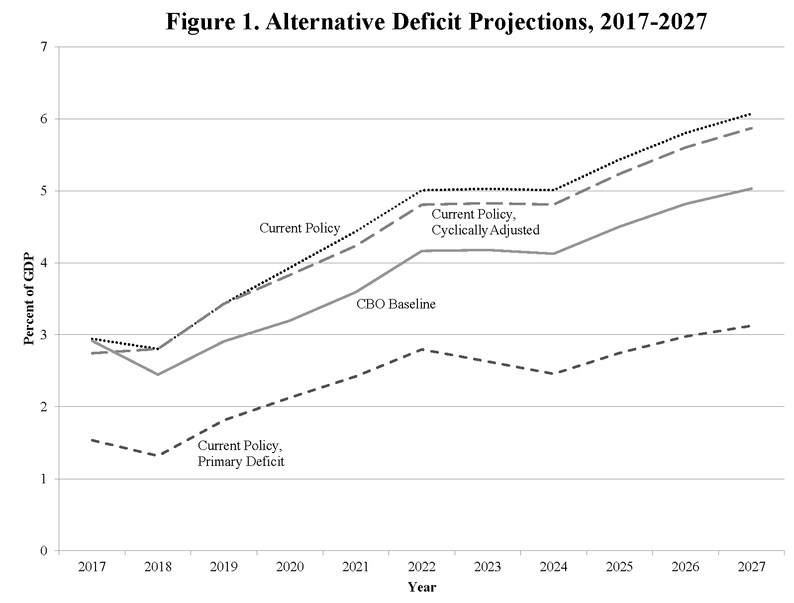
Deficit-GDP and debt-GDP ratios are reported in Figures 1 and 2 and in Appendix Table 1. The deficit, which is 2.9 percent of GDP in 2017, rises to 5.0 percent of GDP in 2027 under current-law and 6.1 percent of GDP under current policy.[2]
The underlying economic projection behind these estimates assumes that the economy remains close to full employment throughout most of the projection period. Figure 1 shows that the cyclically-adjusted deficit (i.e., the deficit with automatic stabilizers removed) rises to 5.9 percent of GDP by 2027. This would be the highest full-employment deficit, other than during the Great Recession, in the post-War period.
Figure 1 also shows that the primary (ex-interest) deficit rises over time. As discussed below, there is some uncertainty over the path that interest rates, and hence net interest payments, will follow. The rising primary deficit shows that there is a growing fiscal shortfall under any positive interest rate scenario.
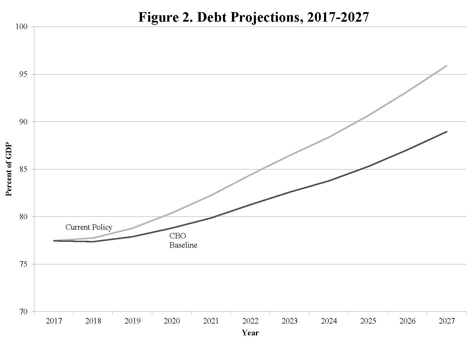
As shown in Figure 2, under current policy, the debt-GDP ratio grows slowly to 80.4 percent of GDP by 2020, after which it starts rising faster to reach 95.9 percent by 2027. The 2027 ratio rises to 88.9 percent under current law.
Given this basic summary, several aspects of the 10-year budget outlook stand out:
- The current debt-GDP ratio is high relative to U.S. historical norms.
At 77 percent, the debt-GDP ratio at the end of 2016 is the highest in U.S. history other than during a seven-year period around World War II. From 1957 to 2007, the ratio never exceeded 50 percent and averaged just 36 percent of GDP. In 2007, the last year before the financial crisis and the Great Recession, the ratio was 35 percent.
- The debt-GDP ratio is projected to rise over the decade, whereas in previous high-debt episodes it fell rapidly.
The debt-GDP ratio rises by more than 18 percentage points from 2017 to 2027 under current policy. This increase occurs despite the projection of a near full-employment economy during this period, hinting at an unsustainable fiscal situation and the need for longer-term analysis. It also highlights the difference between the current situation and previous high-debt episodes in U.S. history. In such episodes – the Civil War, World War I, and World War II – the debt-GDP ratio was cut in half roughly 10 to 15 years after the war ended.
- Total spending is projected to rise over the decade, with the composition shifting significantly.
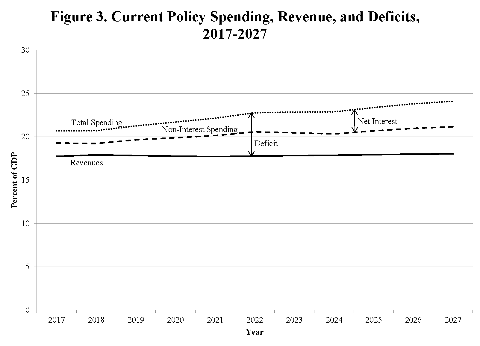
Total spending under current policy rises from 20.7 percent of GDP in 2017 to 24.1 percent by 2027 (Figure 3). This compares to a historical average of 20.0 percent for 1962 to 2016. Net interest payments rise from 1.4 percent of GDP in 2017 to 2.9 percent in 2027. CBO assumes that interest rates will rise significantly as economic growth is maintained.[3] Below, we report budget outlook estimates with lower interest rates.
Non-interest outlays rise by about 2 percent of GDP, with increases in mandatory spending offset in part by declines in discretionary spending. Non-interest spending rises from 19.3 percent of GDP in 2017 to 21.2 percent by 2027. The average value from 1962 to 2016 was about 18.1 percent.
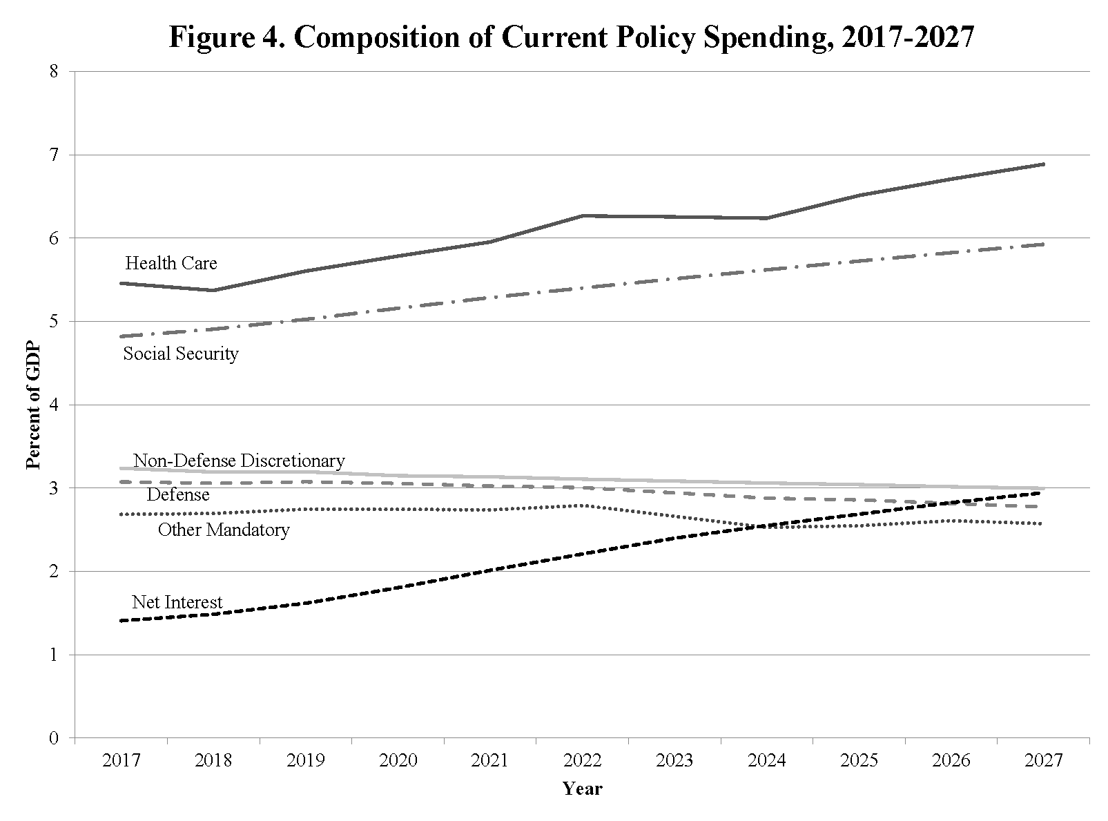
Figure 4 shows the projected composition of spending. Discretionary spending falls from 6.3 percent of GDP in 2017 to 5.8 percent in 2027. Within that category, defense spending declines from 3.1 percent in 2017 to 2.8 percent in 2027, while non-defense discretionary spending falls from 3.2 percent of GDP in 2017 to 3.0 percent of GDP in 2027. All of these shares are low relative to historical figures. Since 1962, the lowest discretionary spending share of GDP occurred in 1999, at 6.0 percent. The lowest share for defense spending was 2.9 percent of GDP in 1999-2001. The lowest nondefense discretionary spending share of GDP was 3.1 percent in 1998-1999.
Under current policy, mandatory spending is projected to rise from 13.0 percent of GDP in 2017 to 15.4 percent in 2027. Spending on Social Security rises by about 1.1 percent of GDP, net Medicare spending rises by 1.1 percent of GDP and Medicaid benefits, CHIP, and exchange subsidies rise by about 0.4 percent of GDP. Other entitlement spending will decline by about 0.1 percent of GDP.
- Revenues are roughly constant as a share of GDP.
Revenues are projected to increase from 17.7 percent of GDP in 2017 to 18.0 percent of GDP in 2027. Revenues averaged 17.4 percent of GDP from 1962 to 2016. Notably, individual income tax revenues are projected to rise from 8.6 percent of GDP currently to 9.7 percent of GDP by 2027 under current policy. The only years in which the income tax has ever raised at least 9 percent of GDP in revenue were 1944 (at the height of World War II), 1981-82 (before the Reagan tax cuts took full effect), and 1998-2001 (helped by a strong economy and the tech stock bubble, and leading to the Bush tax cuts in 2001 and 2003). The increase in individual income tax revenues is offset in part by a decline in corporate taxes from 1.7 percent of GDP in 2017 to 1.3 percent of GDP in 2027. Payroll taxes and other revenues are also projected to drop as a share of the economy over the period.
C. Sensitivity Analysis: The effects of low interest rates
As noted above, CBO’s projections assume rising interest rates over time. The 10-year Treasury rate, for example, is projected to rise from 2.2 percent in 2017 to 3.6 percent in 2023 and remain roughly constant thereafter. However, low interest rates on government debt have proven more persistent than many observers would have guessed at the beginning of the Great Recession. To test the effect of interest rate assumptions on the budget outlook, we adopt an assumption that we believe to be extremely optimistic (for budgetary purposes) – namely, that a weighted average of nominal interest rates on all government debt stays constant at its implied 2017 value (1.9 percent) through 2027.[4] Under this scenario, still assuming current policy for tax and spending programs, we find that in 2027, compared to using CBO interest rate assumptions:
- Net interest payments are 1.6 percent of GDP by 2027, instead of 2.9 percent;
- The deficit rises to 4.7 percent of GDP, instead of 6.1 percent;
- The full-employment deficit rises to 4.5 percent, compared to 5.9 percent;
- Debt rises to 86.3 percent of GDP compared to 95.9 percent.
Thus, lower interest rates improve the 10-year budget outlook, but the debt-GDP ratio is still projected to rise even if interest rates remain at the current level for the next 10 years.
D. Trust funds
The federal government runs several trust funds, most notably for Social Security (Old Age and Survivors Insurance), Disability, Medicare (two separate funds), civilian and military retirement, and transportation spending. All of the projections highlighted above integrate the trust funds into the overall budget. These projections also assume that scheduled benefit payments will be made even if trust funds run their balances to zero. However, many of the trust funds are not legally allowed to pay out benefits that draw their balances below zero.
This is not just an academic concern. This trust-fund constraint was one of the proximate causes of Social Security reform in 1983; the trust fund literally had almost run out of money, an eventuality that would have required cuts in promised benefits so that they would not exceed revenues coming in. The Social Security (Old Age and Survivors Insurance) trust fund is currently scheduled to have to make forced adjustments by 2035. The disability insurance (DI) trust fund is scheduled to have to make forced adjustments by 2023 (Board of Trustees 2016). The Medicare Part A (hospital insurance) fund appears, according to the 2016 Trustees Report, likely to hit a similar constraint by 2028 (Boards of Trustees 2016).
Each of these dates may prompt at least limited fiscal action. In each case, legislators will be forced to override the rules regarding trust funds, make inter-fund transfers, reduce benefits, or raise taxes. In contrast, Social Security (OASI) does not have cash flow issues for a couple of decades and Medicare parts B (Supplementary Medical Insurance) and D (Drug Insurance) do not have the constraint that spending can only be financed by trust fund payments.
Although low trust balances may require action, low balances and actions to address them relate to individual programs and the nature of their funding sources, and provide an incomplete picture of the federal government’s overall fiscal position over the longer term, an issue to which we now turn our attention.
III. The Long-Term Budget Outlook
A. Assumptions
For our long-term current policy model, we assume that most categories of spending and revenues remain constant at their baseline 2027 share of GDP in subsequent years. Assuming constant shares of GDP, however, would be seriously misleading for the major entitlement programs and their associated sources of funding. For the Medicare and OASDI programs, in our base case, we project all elements of spending and dedicated revenues (payroll taxes, income taxes on benefits, premiums and contributions from states) using the intermediate projections in the 2016 Trustees reports.[5] Social Security spending, Medicare spending, and payroll taxes follow the growth rates assumed in the Trustees’ projections of the ratios of taxes and spending to GDP for each year during the 2028–2091 period, assuming that these ratios are constant at their terminal values thereafter. For Medicaid, CHIP, and exchange subsidies, we use growth rates implied by CBO’s most recent long-term static projections (CBO 2016b) through 2046. After 2046, the growth rate is determined by the ratio of pre-2046 annual growth in CBO (2015) versus CBO (2016b), applied to post-2046 annual growth in CBO (2015).[6]
In our base case, we use growth assumptions implied in CBO (2016b). Over the 2028-2046 period, the average nominal economic growth rate is 4.26 percent. After 2046, we assume that the economy grows at its 2046 rate of 4.26 percent. This, again, is due to the Congressional Budget Office (2016b) only reporting data through 2046. In our base interest rate case, we hold the nominal interest rate at its 2027 value of 3.28 percent from 2028-2047. After 2047, we gradually increase the interest rate to 5.17 percent by 2092. This figure represents the long-term nominal interest rate projected by the Board of Trustees (2016), adjusted for differences in economic growth between the trustees’ report and the CBO Long-Term Budget Outlook (CBO 2016b).
By assuming that many categories of tax revenues and spending remain constant relative to GDP, we are not simply projecting based on current law, but instead are assuming that policymakers will make a number of future policy changes, including a continual series of (small) tax cuts, discretionary spending increases, and adjustments to keep health spending from growing too quickly. If current-law tax parameters were extended forward, income taxes would rise as a share of GDP (due to bracket creep and rising withdrawals from retirement plans). If discretionary spending were held constant in real terms, it would fall continually as a share of GDP. Our projection also assumes that a wealthier and more populous society will want to maintain discretionary spending as a share of GDP. We provide sensitivity estimates below.[7]
We provide three projections of Medicare spending. As noted, our base case projections come from the intermediate projections of the Medicare Trustees, which have for many years incorporated the assumption that Medicare growth will eventually slow in the future. Starting in the 2010 report, however, the Trustees’ official medical projections have assumed a much stronger slowdown, as a consequence of provisions in the ACA. These assumptions, though they may be consistent with the impact of the bill’s provisions should they remain in force over the long term, are not adopted by other forecasters, who have a more pessimistic outlook. For example, the Medicare Actuary has, since 2010, released an alternate set of projections showing smaller (although still positive) reductions in spending, which is the source of our second projection. The third projection is the Medicare scenario in CBO’s Long-Term Budget Outlook (2016b), which projects a still more pessimistic path for Medicare spending. The three scenarios generate fairly similar trends for next 30 years – by 2047, the estimates differ by about 1 percent of GDP. Over longer periods, however, the projections diverge significantly; by 2092, the estimates range from 5.2 percent of GDP under the Medicare Trustees’ assumptions to 10.3 percent under CBO’s.[8]
B. Debt Projections
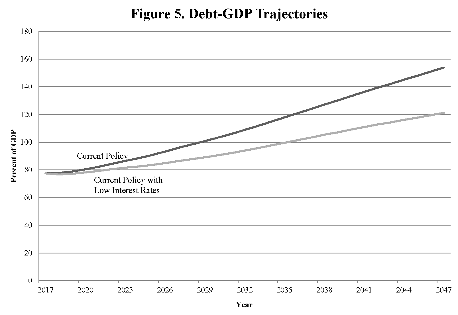
Figure 5 shows the debt trajectory under current policy, using the Medicare Trustees projections for health care (i.e., the lowest of the three health options). The debt-GDP ratio rises from 95.9 percent in 2027, hits 100 percent in 2029, exceeds the previous all-time high of 106 percent in 2032, and rises to 154 percent by 2047 – 30 years from now.
The figure also shows the effect of low interest rates. Specifically, in this scenario we hold interest rates constant at current levels all the way through 2047. Under current policy with low interest rates, the debt-GDP ratio rises to 121 percent by 2047. The debt-GDP ratio continues to rise after 2047 in both scenarios.
C. The Fiscal Gap
The fiscal gap is an accounting measure that is intended to reflect the long-term budgetary status of the government (Auerbach 1994).[9] The fiscal gap answers the question: if you want to start a policy change in a given year and reach a given debt-GDP target in a given future year, what is the size of the annual, constant-share-of-GDP increase in taxes and/or reductions in non-interest expenditures (or combination of the two) that would be required? For example, one might ask what immediate and constant policy change would be needed to obtain the same debt-GDP in 2047 as exists today.[10] Or one might ask, if we wanted the debt-GDP ratio to return to its 1957-2007 average of 36 percent by 2047, what constant-share-of-GDP change would be required starting in 2022?
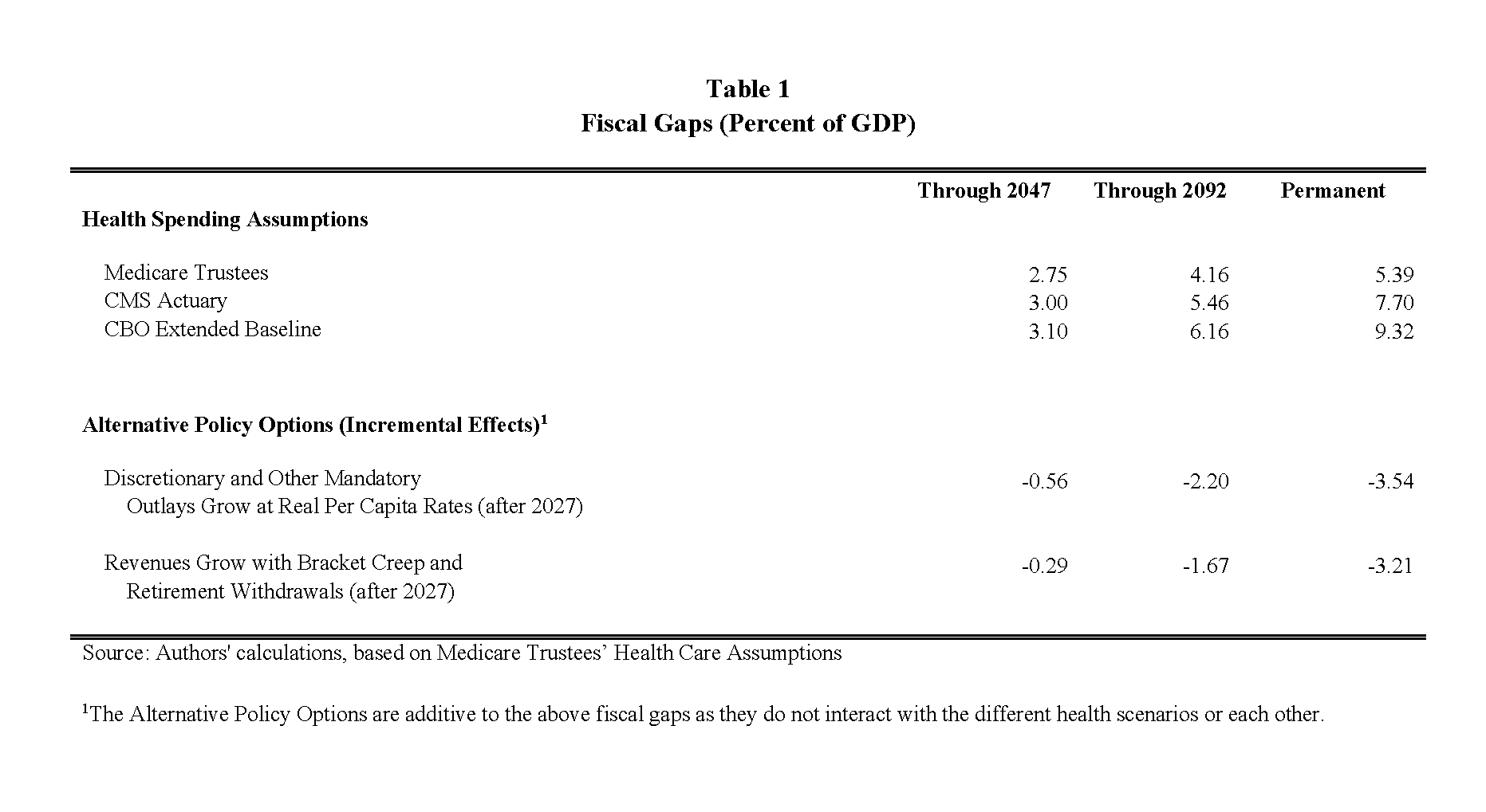
The first row of Table 1 shows fiscal gap estimates using the Medicare trustee projections for health care. We show fiscal gaps for three different horizons, assuming the policy changes begin in 2017, and aiming for the same debt-GDP ratio in the terminal year (77.0 percent of GDP) as existed at the end of 2016. The estimated gap through 2047 is 2.75 percent of GDP. This implies that an immediate and permanent increase in taxes or cut in spending of about $526 billion per year in current terms would be needed to achieve the current debt-GDP ratio in 2047.
The fiscal gap is larger if the time horizon is extended, since the budget is projected to be running substantial deficits in more distant future years. If the horizon is extended through 2092, the fiscal gap rises to 4.16 percent of GDP. If it is extended indefinitely, the gap rises to 5.39 percent of GDP.
The second and third rows of the table show that the choice of health care scenario has a significant and varying impact on the estimated fiscal gaps. Through 2047, the differences in the fiscal gaps implied by the different health care scenarios are relatively small. Over longer periods, however, the differences are much larger. Using the CMS actuaries’ projections instead of the Medicare Trustees’ projections raises the fiscal gap by about 1.3 percent of GDP through 2092 and 2.3 percent of GDP on a permanent basis. Using the CBO Medicare projections raises the gap by an additional 0.7 percent of GDP through 2092 and an additional 1.6 percent of GDP over the infinite horizon.
Related Content


The rest of Table 1 displays a variety of sensitivity analyses concerning policy assumptions. Assuming that outlays for discretionary and other mandatory spending stays constant in real, per capita terms after 2027 (instead of a constant share of GDP) reduces the fiscal gap by about 0.6 percent of GDP through 2047, 2.2 percent of GDP through 2092, and about 3.5 percent of GDP on a permanent basis.
Assuming that net income tax revenues grow with bracket creep after 2027 (instead of remaining a constant share of GDP) reduces the fiscal gap by 0.3 percent of GDP through 2047, 1.7 percent of GDP through 2092, and 3.2 percent of GDP on a permanent basis.
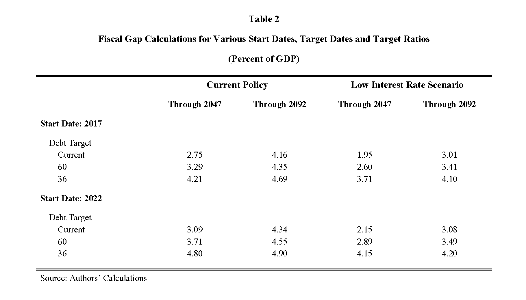
Table 2 shows fiscal gaps under different combinations of debt targets, dates for reaching the target, and dates for implementing the policy changes. We employ three debt targets – 77.0 percent, the ratio of debt-to-GDP at the end of 2016; 60 percent, a ratio proposed by several commissions, including Bowles-Simpson (National Commission on Fiscal Responsibility and Reform 2010) and Domenici-Rivlin (Debt Reduction Task Force 2010), and 36 percent (representing simultaneously (a) the average from 1957-2007, before the Great Recession, (b) roughly the value in 2007 as the financial crisis and Great Recession hit, and (c) a target that cuts the current debt-GDP ratio roughly in half). We look at both 30-year and 75-year target dates for reaching the new debt-GDP level.
We employ two start dates for policy – current (i.e. 2017) and 2022, the latter reflecting the possibility of implementation delays or phase-ins. The first two columns in the first line of Table 2 replicate the fiscal gap calculations through 2047 and 2092 shown in the top row of Table 1, for obtaining a 77.0 percent debt-GDP ratio in the target year, with the policy starting in 2017.
The main message of Table 2 is that it will be quite difficult to return to historical levels of the debt-GDP ratio anytime soon. To get the debt-GDP ratio in 2047 down to 36 percent would require immediate and permanent spending cuts or tax increases of 4.2 percent of GDP. This would require a 24 percent increase in current tax revenues or a 22 percent cut in non-interest spending.
The problem is even harder if the policy does not take effect until 2022. Just maintaining the 2047 debt-GDP ratio at its current level would require annual cuts of 3.1 percent of GDP starting in 2021. Reducing the debt-GDP ratio to 60 percent in 2047 would require cuts 3.7 percent of GDP beginning in 2022. To get the debt-GDP ratio down to 36 percent by 2047 would require deficit reduction of 4.8 percent of GDP per year starting in 2022. To achieve that ratio in 2092 would require cuts of 4.9 percent of GDP starting in 2022.
Holding interest rates at their implied 2017 rate through 2047 does not paint a much better picture, either. Even under this scenario, it would require immediate spending cuts or tax increases of 1.95 percent of GDP just to maintain the current debt ratio through 2047. If the policy were delayed until 2022, the required policy adjustment would be 2.15 percent in order to maintain the current debt-GDP ratio in 2047 and 4.15 percent of GDP in order to reduce the debt-GDP ratio to 36 percent by then. The longer policy makers wait to make the adjustments, the larger the eventual adjustments will have to be.
D. Uncertainty and its Implications
Budget projections are not written in stone. Clearly, they should be taken with a grain of salt – perhaps a bushel. They are, at best, the educated guesses of informed people, and the role of uncertainty in budget projections should not be underestimated, particularly as the time horizon lengthens. In the past, budget projections by CBO and others (including us) have proven to be too optimistic in some instances and too pessimistic at others.
Major sources of uncertainty – noted in the analysis above – include the behavior of interest rates, trends in health care spending, shifts in demographics, and, of course, the choices of policy makers. In each case, the uncertainty can create significant changes in outcomes because errors tend to compound over time. Nevertheless, although there is substantial uncertainty regarding the outlook, reasonable estimates imply an unsustainable fiscal path that will generate significant problems if not addressed.
Related Books


How should the presence of that uncertainty affect when and how we make policy changes? One argument is that we should wait; after all, the fiscal problem could go away. But, for several reasons, ignoring the problem is unlikely to be an optimal strategy.
First, regardless of whether the long term turns out to be somewhat better or worse than predicted, there is already a debt problem. The debt-GDP ratio has already more than doubled, to 77 percent. The future is already here. There are benefits to getting the deficit under control – including economic growth and fiscal flexibility – regardless of whether the long-term problem turns out to be as bad as mainstream projections suggest. If carrying high debt were costless economically and politically, many more countries would have done so before the Great Recession. In fact, very few had net debt to GDP ratios above 70 percent.
Second, purely as a matter of arithmetic, the longer we wait, the larger and more disruptive the eventual policy solutions will need to be, barring a marked improvement in the fiscal picture. Note that addressing the issue now does not necessarily mean cutting back on current expenditures or raising current taxes substantially or even at all; rather, it may involve addressing future spending and revenue flows now, in a credible manner.
Third, uncertainty can cut both ways and the greater the uncertainty the more we should want to address at least part of the problem now. The problem could turn out to be worse – rather than better – than expected, in which case delay in dealing with the problem would make solutions even more difficult politically and even more wrenching economically. If people are risk-averse, the existence of uncertainty should normally elicit precautionary behavior – essentially “buying insurance” against a really bad long-term outcome by reducing the potential severity of the problem – through enactment of at least partial solutions to the budget problem right away.[11]
IV. Conclusion
Although current deficits are reasonably low, the medium- and long-term fiscal outlook is nevertheless troubling. Even under a low interest rate scenario, the long-term budget outlook is unsustainable. Moreover, the nation already carries a debt load that is more than twice as large as its historical average as a share of GDP, and that makes evolution of the debt-GDP ratio much more sensitive to interest rates.
The necessary adjustments will be large relative to those adopted under recent legislation. Moreover, the most optimistic long-run projections already incorporate the effects of success at “bending the curve” of health care cost growth, so further measures will clearly be needed.[12] These changes, however, relate to the medium- and long-term deficits, not the short-term deficit.
Looking toward policy solutions, it is useful to emphasize that even if the main driver of long-term fiscal imbalances is the growth of entitlement benefits, this does not mean that the only solutions are some combination of benefit cuts now and benefit cuts in the future. For example, when budget surpluses began to emerge in the late 1990s, President Clinton devised a plan to use the funds to “Save Social Security First.” Without judging the merits of that particular plan, our point is that Clinton recognized that Social Security faced long-term shortfalls and, rather than ignoring those shortfalls, aimed to address the problem in a way that went beyond simply cutting benefits. A more general point is that addressing entitlement funding imbalances can be justified precisely because one wants to preserve and enhance the programs, not just because one might want to reduce the size of the programs. Likewise, addressing these imbalances may involve reforming the structure of other spending, raising or restructuring revenues, or creating new programs, as well as simply cutting existing benefits. Nor do spending cuts or tax changes need to be across the board. Policy makers should make choices among programs. For example, more investment in infrastructure or children’s programs could be provided, even in the context of overall spending reductions.
References
Auerbach, Alan J. 1994. “The U.S. Fiscal Problem: Where We Are, How We Got Here, and Where We’re Going.” In National Bureau of Economic Research Macroeconomics Annual 1994, Volume 9, edited by Stanley Fischer and Julio Rotemberg, 141–175. Cambridge, MA: MIT Press.
Auerbach, Alan J. 1997. “Quantifying the Current U.S. Fiscal Imbalance.” National Tax Journal 50 (3): 387–98.
Auerbach, Alan J. 2014. “Fiscal Uncertainty and How to Deal with It.” Hutchins Center, Brookings Institution, Washington, DC.
Auerbach, Alan J., William G. Gale, Peter R. Orszag, and Samara Potter. 2003. “Budget Blues: The Fiscal Outlook and Options for Reform.” In Aaron, Henry J., James Lindsay, and Pietro Nivola (eds.), Agenda for the Nation, 109–143. Brookings Institution, Washington, DC.
Board of Trustees, Federal Old-Age and Survivors Insurance and Disability Insurance Trust Funds. 2016. The 2016 Annual Report of the Board of Trustees of the Federal Old-Age and Survivors Insurance and Federal Disability Insurance Trust Funds. Federal Old-Age and Survivors Insurance and Disability Insurance Trust Funds, Washington, DC.
Boards of Trustees, Federal Hospital Insurance and Federal Supplemental Medical Insurance Trust Funds. 2016. The 2016 Annual Report of the Board of Trustees of the Federal Hospital Insurance and Federal Supplemental Medical Insurance Trust Funds. Federal Hospital Insurance and Federal Supplemental Medical Insurance Trust Funds, Washington, DC.
Congressional Budget Office. 2015. “The 2015 Long-Term Budget Outlook.” Congressional Budget Office, Washington, DC.
Congressional Budget Office. 2016a. “An Update to the Budget and Economic Outlook: 2016 to 2026.” Congressional Budget Office, Washington, DC.
Congressional Budget Office. 2016b. “The 2016 Long Term Budget Outlook.” Congressional Budget Office, Washington, DC.
Congressional Budget Office. 2017. “The Budget and Economic Outlook: 2017 to 2027.” Congressional Budget Office, Washington, DC.
Authors