Update on the structure of US Treasury debt from a model’s perspective

Introduction

In Optimizing the Maturity Structure of U.S. Treasury Debt: A Model Based Framework, a 2018 Hutchins Center working paper, Belton et al. presented an optimal debt management model for U.S. Treasury debt managers to consider, alongside other inputs, as they make decisions on issuance across maturities and instruments, as well as about the ultimate structure of Treasury’s outstanding debt.¹

Belton et al. endorsed Treasury’s long-standing principle of acting as a “regular and predictable” issuer but noted that this principle “does not specify the ultimate maturity structure that best serves the U.S. Treasury.” The model focuses on the trade-off the debt manager must consider between the expected cost of interest payments on the debt and the variability of the deficit arising from those interest payments. In particular, issuing shorter-term debt could lower the expected cost of the debt but also involves greater deficit variability, as interest payments on the debt would fluctuate more widely. Issuing longer-term debt could involve a somewhat higher cost on average but also could result in less variation in deficits in some circumstances. The model can calibrate that trade-off under a given set of assumptions and thereby assess the optimality of different maturity structures for Treasury debt.

The importance of these debt management decisions is evident. In 2025, the federal government is projected to spend nearly $1 trillion on debt service, making it one of the largest items in the federal budget. Choosing a debt structure that is expected to keep this debt service cost as low as possible is crucial. But allowing too much variability in that cost introduces additional risk into fiscal planning—if the cost of funding the debt were to unexpectedly shift higher, Congress and the president would be faced with making tough choices between running a higher-than-expected deficit or else making adjustments through spending cuts or tax increases.

As the authors of that paper discussed, an important consideration in using the model is that it makes assumptions about the behavior of the economy, the fiscal outlook, and market dynamics—all of which are uncertain and change over time. A presentation by the Treasury Borrowing Advisory Committee (TBAC) in 2023 considered how the environment surrounding debt management decisions had changed since 2018 and explored how particular assumptions from the model are important to the model’s recommendations. In this post, we reflect on the results from that TBAC presentation, drawing from our experience developing and using the underlying model, to provide an updated view on debt management issues facing the U.S. Treasury.

Our conclusion, through the lens of the debt model, is that the current structure of the debt is efficient for a debt manager that exhibits a relatively high degree of concern about deficit variation. Shifting Treasury issuance more aggressively towards the long end of the curve is likely to result in increased funding costs that would be difficult to justify by the corresponding modest reduction in deficit variability unless the debt manager exhibits extreme risk aversion.

An important caveat to that conclusion, however, is that it is sensitive to the evolution of the term premium embedded in the Treasury curve. (The term premium, as explained below, is the extra yield realized on longer-term Treasuries above short-term Treasuries, on average.) If the debt manager believes that the term premium in the future will tend to be lower than had been the case historically, then it could be attractive to move more issuance longer on the curve. If the term premium is expected to be consistent with history, as is assumed in the model, then the preference would be to focus issuance in short- and intermediate-term maturities.

Shift in the environment for debt management

The macro environment has changed significantly since 2018, notably because of the macroeconomic consequences of the COVID pandemic and the corresponding fiscal and monetary policy responses. We consider how some of those changes affect the model’s output and the implied recommendations for the debt managers.

Among the most dramatic changes in the macro environment in recent years has been the path of inflation. The model’s structure assumes that a surge in inflation would mean revert over time because of the policy response of the Federal Reserve. The model’s anticipation of that mean reversion has mostly been realized, as evidenced by both recent inflation data and inflation expectations implied from survey and market pricing.

In contrast, a development that seems unlikely to revert in the foreseeable future is the significantly increased stock of outstanding Treasury debt and the prospect for large fiscal deficits going forward.  Debt held by the public as a share of GDP increased from 78.4% in 2019 to 97.1% by the fourth quarter of 2024. Moreover, projections for deficits over the next decade have grown substantially larger than had been forecast prior to COVID, implying that the debt stock is expected to continue to increase meaningfully as a share of GDP.

Implications for the trade-off faced by Treasury

This shift in the fiscal outlook has important implications for debt management. We begin by looking at the evolution of the situation facing debt managers from 2019Q4, just before COVID, compared to a post-pandemic quarter, 2023Q1.

Our analysis starts with model results utilizing a single-issue strategy to demonstrate how the model operates. By construction, a single-issue strategy assumes that debt managers fund the entire debt at a single point on the curve. Such an approach is of course unrealistic—funding the entire debt with a single tenor would not be feasible or optimal—but the results are illustrative of the model’s behavior.

The results are shown in Figure 2, where the vertical axis on each chart is the average debt service cost as a percent of GDP, and the horizonal axis is the variability (the standard deviation) in the deficit (inclusive of debt service cost) as a percent of GDP, both measured at a 20-year horizon.

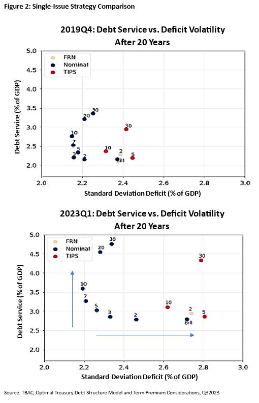
The most dramatic change in the model results is that the frontier of outcomes that the debt manager could achieve has deteriorated substantially, shifting up and to the right. The higher debt stock makes debt service more costly on average as a share of GDP (points moved upward), and it exacerbates the variability of the deficit (points moved to the right).

Regarding the trade-offs among specific maturities, we can make several observations that are true in both the pre- and post-pandemic scenarios. The lowest cost achieved on average across the nominal securities (the blue dots) is for bills and short-term coupon securities, while longer-term securities are notably more expensive. This pattern is driven by the model’s term premium assumptions, as the term premium is expected to be positive on average, as discussed in more detail below. However, shorter maturities also imply a larger variability in the deficit compared to other nominal securities. Moreover, this effect on deficit variability is now even more acute, given the substantial increase in the size of the debt stock.²

A debt manager could choose the point on the frontier that achieves the best trade-off between expected cost and variability of deficits based on the government’s risk preferences. For plausible risk preferences, the model continues to favor issuance of intermediate maturities, as they reduce variability without sharply increasing funding cost. A significant difference from 2019 to consider is that front end issuance is now relatively less attractive compared to intermediate maturities. Most notably, bills and two-year Treasuries now introduce substantially more deficit variability than previously had been the case, while issuing at modestly longer maturities appears more attractive.

Effects of various changes in debt issuance patterns

Of course, Treasury implements its issuance strategy across a range of maturities and security types rather than at single issuance points, so we now turn to more realistic issuance strategies. We do so by using the issuance kernels from the original paper, but expanded to include issuance of TIPS (Treasury Inflation Protected Securities) and FRNs (Floating Rate Notes).³

By varying issuance across these kernels, we can again derive a frontier of possible trade-offs that the debt manager could achieve, only now with more realistic issuance patterns. This new frontier sits modestly lower (lower cost) and to the left (lower variability) compared to the single-strategy frontier, which makes sense as the Treasury gets diversification benefits from issuing across the curve.

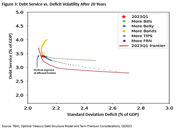
The frontier itself (pink line) has a similar shape as the single-issuance frontier. If the debt manager is willing to tolerate slightly higher variation in deficits, allowing the standard deviation to rise from 2.1% of GDP to 2.2%, the manager can achieve a substantial reduction in average debt service cost, from approximately 3.5% of GDP to 3.0%. To push debt service cost down further, however, the debt manager would need to be willing to accept much greater volatility of deficits, reflecting the convex shape of the frontier. 

The red star on the chart indicates the debt structure that would have been achieved under the 2023Q1 issuance patterns. One immediate observation is that this issuance pattern produces a debt structure that is not far from the frontier—debt issuance appears fairly efficient in this sense. However, the part of the frontier that it is nearest is quite vertical, suggesting that reducing variability would come at a relatively high cost, but that tolerating modest increases in variability could result in meaningful cost savings.

Starting from the 2023Q1 point (the red star), we can measure the changes to debt outcomes if issuance is changed in various directions, as captured by the lines moving from that point in various directions.  For example, the dotted green line shows the impact of increasing bill issuance, which is to lower debt service cost but increase volatility. The results indicate that increasing bills and/or increasing “belly issuance” (the two- to ten-year sector) would move the trade-off down and to the right in a manner that tracks the shape of the frontier. How far the debt manager would choose to move in that direction depends on the degree of risk aversion of the debt manager.

In contrast, issuing more bonds does not look attractive. It involves incurring higher cost with little reduction in variability, moving up the vertical segment of the frontier; eventually it bends back towards greater variability, a lose-lose outcome for the debt manager.

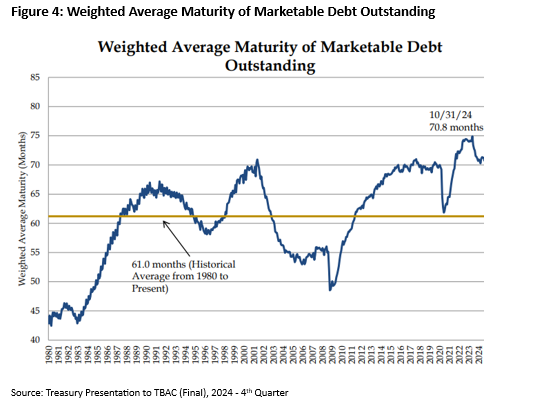
These results provide some perspective on the recent policy discussion about long-end issuance. Some have suggested the Treasury missed an opportunity to term out its debt at low rates before 2022. But given that Treasury’s debt management is designed to be regular and predictable, a decision to introduce additional long-term Treasury tenors or to issue much more heavily in the long end would have been implemented gradually and likely remained in place for many years. Thus, even if Treasury would have managed to lock in low rates during a two-year window, that would ultimately comprise only a modest portion of Treasury’s total long-end debt, and it would have subsequently left Treasury with an issuance pattern skewed heavily toward the long-end. The above model results indicate that this pattern would involve substantial costs over time. It is also worth noting that the issuance pattern chosen by the Treasury debt managers has resulted in the weighted-average-maturity (WAM) of Treasury debt being quite high in recent years relative to the historical average.

An alternative is that Treasury could have moved away from its regular and predictable approach and termed out substantially more of its debt. In evaluating that approach, one must consider market implications. If Treasury were to opportunistically flood the market with long end issuance when rates appear low, the term premium would likely increase considerably in response. Such a change would also sacrifice the long-term cost reduction benefit Treasury accrues by hewing to its principle of regular and predictable debt issuance.

Returning to the model, one may wonder what it would take to not just move down and to the right through increased bill and belly issuance, but to actually reach the frontier in that region. The model does not require an unrealistic clumping of issuance in any specific part of the curve to reach the frontier. What it does call for is increased issuance in the belly (particularly 7- and 10-year maturities) combined with decreases in both the front-end (bills through 3-year maturity) and the long-end (20- and 30-year maturities).  

The importance of the term premium

The term premium is a measure of the expected extra return (above that achieved from rolling over short-term investments such as Treasury bills) investors earn for holding the additional duration risk of longer-term securities. Term premium proves to be a critical concept for debt managers as well, as it captures the extra cost that the Treasury incurs by pushing issuance into longer maturities, Treasury’s extra cost being the flip side of the extra return to investors.

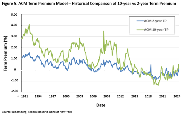
The model assumes the 10-year term premium over time moves towards a level of +50 basis points (bps), while the 2-year term premium tends to be 0 bps. When the term premium differs from those levels, the model assumes that over time the term premium will converge back to +50 and 0.⁴

Those assumptions are based on the historical properties of the Adrian, Crump, and Moench (ACM) model, which is the term structure model imposed on the optimal debt management model. As shown below, the 10-year term premium (green) was consistently above the 2-year term premium (blue) for several decades up to 2017—just before the Belton et al. paper was published. For the most recent five-year period, however, the slope of the term structure has been about flat on average.

The intention of the optimal debt management model was to avoid taking an aggressive stand on the term premium. Rather, the model relies on a generally well-respected term premium model already in the public domain as one of many inputs into a process designed to provide useful guidance to debt managers about debt issuance trade-offs. But given that the levels of the term premium can vary in a manner that at times show considerable persistence, it is difficult to know how to set these term premium assumptions. As a result, it is prudent for debt managers to consider the impact on the model results of an alternative term premium assumption.

Rather than assume these term premia mean revert to the historical norm, the 2023 TBAC analysis considers an alternative scenario in which the expected 10-year term premium is significantly lowered, with the gap between the 10-year and 2-year compressed, and with other points along the curve extrapolated accordingly. While this low term premium assumption still incorporates a modest amount of term premium along the curve, it is considerably less than that observed in the longer-term history or in the model’s standard assumption. The resulting debt management frontier is shown in Figure 6 (right), side-by-side with the standard model term premium assumption (left). The frontier shifts down notably, as one would expect, as the reduced term premium implies lower long-end financing costs. More importantly, the effects of various debt management decisions flatten out significantly. Essentially, it becomes less consequential for expected cost which maturity points are issued; as such, the cost of reducing deficit volatility by further terming out the debt becomes smaller.

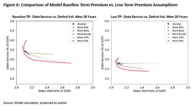
If the term premium tends to be quite low and importantly is expected to remain low indefinitely, then long-term debt is not much more costly than short-term debt on average, and the debt manager should choose a debt mix that includes a greater share of longer-term debt than it would have otherwise. However, there are reasons to be skeptical of this assumption. First, the term premium has been moving notably higher of late. And second, comparing Treasuries to swap rates points to a higher relative funding cost for the longer end: The 30-year Treasury yield is currently about 80 bps higher than a comparable swap rate, compared to about 15bps for the 2-year Treasury. Since this spread is a part of the term premium on Treasury securities, a very low term premium assumption across the curve does not seem plausible.

Conclusions

This analysis indicates that debt managers face a more difficult situation now than when the Belton et al. paper was published in 2018 given the large increase in the debt. Both the expected cost of the debt and the variability of budget deficits are now much higher. To move closer to the frontier implied by the model, debt managers could incrementally increase issuance in the belly of the curve, while reducing issuance in both front-end and long-end maturities.

Treasury chose to increase the WAM of its outstanding debt in the period of low rates triggered by the pandemic. However, skewing a higher share of future increases in debt issuance toward long-term maturities will not provide an effective trade-off between funding cost and risk reduction if the term premium increases toward historical (pre-2017) norms. Expectations about the path of the term premium will be critical for determining the most effective approach taken by debt managers.